Theorem 1: If $n>2$ is an integer, there is no dominant rational map from $\mathbb{P}_{\mathbb{C}}^1$ to the curve cut out by $x^n+y^n=z^n$ in $\mathbb{P}_{\mathbb{C}}^2$.

The curve cut out by $x^n+y^n=z^n$ in $\mathbb{P}_{\mathbb{C}}^2$ is called the Fermat curve, and we will often denote it by $F_{\mathbb{C}}^n$. More generally, we will use the notation $F_{k}^n$ if we are working over the base field $k$.

We will discuss two different ways to prove this. The first is a lowbrow method, relying on some explicit manipulation of polynomials. We will then see that this result follows more abstractly from invariants of curves.

Lowbrow Proof

This is a proof by infinite descent that uses some clever algebra to generate polynomial solutions to Fermat’s equation of strictly smaller degree, given some starting solutions.

Proof of Theorem 1: Suppose there exists a dominant rational map $\varphi\colon\mathbb{P}_{\mathbb{C}}^1\dashrightarrow F_{\mathbb{C}}^n$ from the projective line to the Fermat curve, where $n>2$. After dehomogeneization in an affine chart, this rational map should be given by the data of three rational functions $f(t)$, $g(t)$, and $h(t)$, satisfying the equation $f(t)^n+g(t)^n=h(t)^n$. By Theorem II.6.8 of Hartshorne, since the projective line is a complete curve, it follows that the image of $\varphi$ is either a point or $F_{\mathbb{C}}^n$ itself. Since this map is dominant, we note that the image of $\varphi$ cannot be a single point. That is, the rational functions $f(t)$, $g(t)$, and $h(t)$ should not be constants. Clearing denominators and canceling common factors, we obtain polynomials $F(t)$, $G(t)$, and $H(t)$ that are relatively prime and satisfy $F(t)^n+G(t)^n=H(t)^n$.

Suppose furthermore that the polynomials $F$, $G$, and $H$ solving Fermat’s equation are chosen so that $\min{(\deg{F},\deg{G})}$ is minimal amongst all tuples of polynomial solutions to Fermat’s equation. Without loss of generality, let us assume that $\deg{F}=\min{(\deg{F},\deg{G})}$. Note that

where $\zeta$ is a primitive $n$^th root of unity. We claim that each factor $H(t)-\zeta^jG(t)$ is itself an $n$^th power. Indeed, note that if $H(t)-\zeta^jG(t)$ and $H(t)-\zeta^kG(t)$ share a common factor for $j\neq k$ (with $1\leq j,k\leq n$), they must also share a common root. Evaluation of both factors at that root then forces either $H$ and $G$ to share a common factor, or $\zeta^j=\zeta^k$, a contradiction in either case. Hence, each factor in our factorization above has distinct factors. Since the product above is itself an $n$^th power, namely $F(t)^n$, and $\mathbb{C}[t]$ is a UFD, it must be the case that each factor must be an $n$^th power as claimed.

Now consider the system of equations

The solution to this system of equations is given by $\alpha = -\frac{\zeta + 1}{\zeta}$ and $\beta = -\frac{1}{\zeta}$. By construction, we have that

We have already shown that each factor in the brackets is itself an $n$^th power. Therefore, we may define the polynomials $\tilde{F}(t)=\left[H(t)-G(t)\right]^{1/n}$, $\tilde{G}(t)=\alpha^{1/n}\left[H(t)-\zeta G(t)\right]^{1/n}$, and $\tilde{H}(t)=\beta^{1/n}\left[H(t)-\zeta^2 G(t)\right]^{1/n}$, and they will satisfy $\tilde{F}(t)^n+\tilde{G}(t)^n=\tilde{H}(t)^n$. Since $n>2$, we have that $\alpha$ and $\beta$ are both nonzero, so all three of these new polynomials are nonconstant. But by construction, the degrees of $\tilde{F}$ and $\tilde{G}$ are both strictly less than the degree of $F$, contradicting the minimality of $\min{(\deg{F},\deg{G})}$. $\square$

Notice that the proof above fails for $n=2$ because that would force $\alpha=0$ and so $\tilde{G}=0$.

The heart of what we have shown is that no polynomials satisfy Fermat’s equation $F(t)^n+G(t)^n=H(t)^n$ for $n>3$. This is sometimes called Fermat’s last theorem for polynomials. The linked file offers three approaches to this. The first one is essentially what we have shown above. We will expand more on the third approach which is more abstract and geometric in nature. Our proof above heavily relies on the complex numbers, but much of the geometric approach will work more generally over any base field.

Highbrow Proof

The main piece of technology we need to discuss is the Riemann–Hurwitz theorem. But before we do this, let us discuss in more detail how dominant rational maps of the kind we are interested in actually promote to genuine morphisms. The main result is the following.

Theorem 15.3.1, Curve-to-Projective Extension, (Vakil): Suppose $C$ is a pure dimension $1$ Noetherian scheme over an affine base $S=\operatorname{Spec}{A}$, and $p\in C$ is a regular closed point of it. Suppose $Y$ is a projective $S$-scheme. Then any morphism $C\setminus\{p\}\to Y$ of $S$-schemes extends to all of $C$.

Applying this theorem inductively, we can see that under the same hypotheses, a morphism from the complement of any finite set of regular closed points will extend to all of $C.$

The projective line is certainly a pure dimension $1$ Noetherian scheme. The Fermat curve over a field $k$ is a projective $k$-scheme (see Definition 4.5.10 of Vakil). A rational map $\mathbb{P}_k^1\dashrightarrow F_{k}^n$, for any $n$ can be represented by a genuine morphism defined on some open subset $U\subseteq\mathbb{P}_k^1$. But the Zariski topology on $\mathbb{P}^1$ is quite simple and such a subset is simply the complement of some finite collection of closed points (and all closed points of projective space are regular). By the theorem above, this representative will then extend uniquely to a morphism defined on all of $\mathbb{P}_k^1$. Therefore, the existence of a dominant rational map $\mathbb{P}_k^1\dashrightarrow F_{k}^n$ is really just equivalent to the existence of a surjective morphism $\mathbb{P}_k^1\to F_{k}^n$. This is important for us since Riemann–Hurwitz does not directly apply to rational maps between curves, but instead works for certain kinds of morphisms.

Now we need to understand something about the topology of the curves involved in our question. A basic topological property of the projective spaces is that they are irreducible. We can also show that over most fields, the same is true of the Fermat curve for any $n$.

Lemma 1: Let $n$ be a positive integer and let $k$ be a field whose characteristic does not divide $n$. The Fermat curve $F_k^n$ is irreducible.

Proof: We need to show that $x^n+y^n-z^n$ is irreducible in $k[x,y,z]$.

Note that the polynomial $T^n-1\in k[T]$ has formal derivative $nT^{n-1}$. Since the characteristic of $k$ does not divide $n$, this formal derivative is not the zero polynomial, and so it does not share any roots with $T^n-1$ in the algebraic closure $\overline{k}$ of $k$. Hence there are $n$ distinct $n$^th roots of unity in $\overline{k}$. Note that the factorization

where product ranges over all $n$^th roots of unity in $\overline{k}$ counted with multiplicity, holds purely formally by Vieta’s formulas. Since there are $n$ distinct $n$^th roots of unity, it follows that this factorization consists of $n$ distinct linear factors, and so this is the irreducible factorization of $y^n-z^n$ in $\overline{k}[y,z]$.

In particular, if we fix a root of unity $\zeta$, then $y-\zeta z$ is an irreducible factor of $y^n-z^n$ in the ring $\overline{k}[y,z][x]$ whose square does not divide $y^n-z^n$. Since $\overline{k}[y,z][x]$ is a UFD, it follows that $\langle y-\zeta z\rangle$ is a prime ideal, and $y^n-z^n\notin\langle y-\zeta z\rangle^2$. Of course, $1\notin \langle y-\zeta z\rangle$ and $y^n-z^n\in \langle y-\zeta z\rangle$, so $x^n+y^n-z^n$ is irreducible in $\overline{k}[y,z][x]\cong\overline{k}[x,y,z]$ by the generalized Eisenstein’s criterion. Hence, it is irreducible over $k[x,y,z]$. $\square$

Of course, working in the algebraic closure of $k$ in the proof above is overkill—it suffices to work in the splitting field of $T^n-1$. Also note that the condition that the characteristic of $k$ does not divide $n$ is essential. Suppose that $p=\operatorname{char}{k}$. Since the freshman’s dream is valid in prime characteristic, if $p\mid n$ we would have the factorization $x^n+y^n-z^n=(x^{n/p}+y^{n/p}-z^{n/p})^p$.

The topological data that breaks the problem open is the genus of the curves.

Definition 1: Let $X$ be a nonsingular variety and let $\omega_X$ be its canonical bundle. The geometric genus of $X$ is defined to be the zeroth Betti number of $\omega_X$, denoted $g(X):=h^0(X,\omega_X)$.

Since the zeroth sheaf cohomology is just the space of global sections, we can also think of the geometric genus as the dimension of the space of global sections of the canonical bundle. We first show how to compute the geometric genus of $\mathbb{P}^1_k$ by finding its canonical bundle in two different ways.

Theorem 2: $g(\mathbb{P}^1_k)=0$.

Proof 1 of Theorem 2: Consider the standard affine charts $U_0=\operatorname{Spec}{k[x_{1/0}]}$ and $U_1=\operatorname{Spec}{k[x_{0/1}]}$ of the projective line, with the change of coordinates given by $x_{1/0}=\frac{1}{x_{0/1}}$. The affine line has cotangent bundle $\Omega_{k[x]/k}\cong\mathcal{O}_{\mathbb{A}^1_k}$, which is a line bundle. Therefore, the cotangent bundle $\Omega_{\mathbb{P}^1_k/k}$ must be a line bundle. That is, we must have $\omega_X=\Omega_{\mathbb{P}^1_k/k}\cong\mathcal{O}_{\mathbb{P}_k^1}(m)$ for some integer $m$.

Consider the section $dx_{1/0}$ of the cotangent bundle over $U_0$. Since $x_{1/0}=\frac{1}{x_{0/1}}$, we have the relation $dx_{1/0}=-\frac{1}{x_{0/1}^2}\, dx_{0/1}$, hence this section has a pole of order $2$ in $U_0$ wherever $x_{0/1}=0$. It follows that $\Omega_{\mathbb{P}^1_k/k}\cong\mathcal{O}_{\mathbb{P}_k^1}(-2)$. This sheaf has no nonzero global sections, hence $g(\mathbb{P}^1_k)=0$ as claimed. $\square$

We can also calculate the genus of the projective line without getting our hands dirty by using the Euler sequence.

Proof 2 of Theorem 2: We first write the Euler sequence:

Now we take determinants in this short exact sequence (using Exercise 7.29 of Görtz–Wedhorn or Exercise 5.16(d) of Hartshorne). This yields

We have $\omega_{\mathbb{P}^1_k}=\det{\Omega_{\mathbb{P}^1_k/k}}$ and $\det{\mathcal{O}_{\mathbb{P}^1_k}}\cong \mathcal{O}_{\mathbb{P}^1_k}$. Hence, the above becomes

So just as before, we have $g(\mathbb{P}^1_k)=0$ as claimed. $\square$

Arithmetic Genus

Calculating the geometric genus of the Fermat curve will be harder. To do this, we will instead calculate a different invariant, the arithmetic genus, and then see that in the smooth case the two invariants should match.

Definition 2: Let $X$ be a scheme of dimension $n$. The arithmetic genus of $X$ is defined to be $p_a(X):=(-1)^n(\chi(X,\mathcal{O}_X)-1)$.

It turns out the arithmetic genus looks a lot simpler in the case of an integral projective curve over an algebraically closed field (such as a compact Riemann surface). To show this, we first need the following lemma which is an algebraic generalization of Liouville’s theorem.

Lemma 2: Let $k$ be an algebraically closed field and let $X$ be a connected, reduced, proper $k$-scheme. Then the only global functions on $X$ are the constant functions: $\Gamma(X,\mathcal{O}_X)=k$.

Proof: This argument is given by 11.4.7 in Vakil. Let $f\in\Gamma(X,\mathcal{O}_X)$ be a global function on $X$. Recall that morphisms $X\to\mathbb{A}_k^1$ are in correspondence with ring homomorphisms $k[t]\to\Gamma(X,\mathcal{O}_X)$, which by evaluation at $t$ are in “$\sharp$-correspondence” with global functions in $\Gamma(X,\mathcal{O}_X)$ (see 7.6.1 of Vakil). Let $\pi\colon X\to\mathbb{A}_k^1$ be the morphism corresponding to $f$ under this correspondence. Let $\iota\colon\mathbb{A}_k^1\hookrightarrow\mathbb{P}_k^1$ be the standard open embedding.

We know that $\mathbb{P}_k^1$ is separated over $k$ (Vakil 11.2.8) and $X$ is proper over $k$ by assumption, hence by Proposition 11.4.4(e) of Vakil/Corollary II.4.8 of Hartshorne, it follows that the composition $\iota\circ\pi$ is proper. In particular, the composition is closed. Since $X$ is connected, it follows that the image of $\iota\circ\pi$ is a closed, connected subset of $\mathbb{P}_k^1$, so the image is either a single closed point or all of $\mathbb{P}_k^1$. But the embedding $\iota$ is not surjective, so the image of $\iota\circ\pi$ must be a single closed point. In particular, this must be a closed point of $\mathbb{A}_k^1$, and such a point can be identified with an element $p\in k$ since $k$ is algebraically closed.

Since $X$ is reduced and the point $p$ is closed, Corollary 9.4.5 and Exercise 9.4.A of Vakil imply that the scheme-theoretic image of $\pi$ is exactly $p$ with the reduced structure. This means $\pi$ factors as the composition of the structure morphism $X\to\operatorname{Spec}{k}$ and the closed embedding $\operatorname{Spec}{k}\hookrightarrow\mathbb{A}_k^1$ which identifies $\operatorname{Spec}{k}$ with the closed point $p$. By the functoriality of the $\sharp$-correspondence, it follows that $\pi$ corresponds exactly to the global section $f\in\Gamma(X,\mathcal{O}_X)$ which is equal to the constant map $k[t]\to k$ sending $t\mapsto p$, composed with the ring homomorphism $k\to\Gamma(X,\mathcal{O}_X)$ induced by the structure morphism of $X$. $\square$

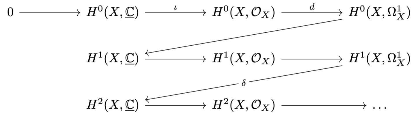
The upshot of Lemma 2 is that if $X$ is an integral projective curve over an algebraically closed field (like a compact Riemann surface), then $h^0(X,\mathcal{O}_X)=1$. Then the arithmetic genus of $X$ simplifies to the first Betti number: $p_a(X)=h^1(X,\mathcal{O}_X)$. Let us specialize even further to the case that $X$ is a connected, compact Riemann surface. Let us further assume the GAGA miracle that the Betti numbers of the sheaf of algebraic functions on $X$ match the Betti numbers of the sheaf of holomorphic functions on $X$. Then due to the Hodge decomposition on the cohomology of $X$, we have that the topological Euler characteristic is

But recall that the topological Euler characteristic equals $2-2g$ for closed orientable surfaces, where $g$ is the topological genus. Hence the arithmetic genus is equal to the topological genus of $X$! So it is not entirely unfair to consider the quantity $p_a(X)$ a type of “genus”. Let us push further and argue that in the case we are interested in, the arithmetic genus will agree with the geometric genus.

Theorem 3: Let $X$ be a smooth irreducible projective curve. Then $g(X)=p_a(X)$.

Proof: This follows immediately from Serre duality:

$\square$

Hence in the case of a connected, compact Riemann surface, the topological genus equals the arithmetic genus, which equals the geometric genus. This gives another justification for Theorem 2 in the case that $k=\mathbb{C}$, since the projective line $\mathbb{C}P^1$ is topologically the sphere $S^2$ which has genus $0$. More generally, orientable compact connected surfaces are classified to be the connected sums of tori with the sphere as shown below.

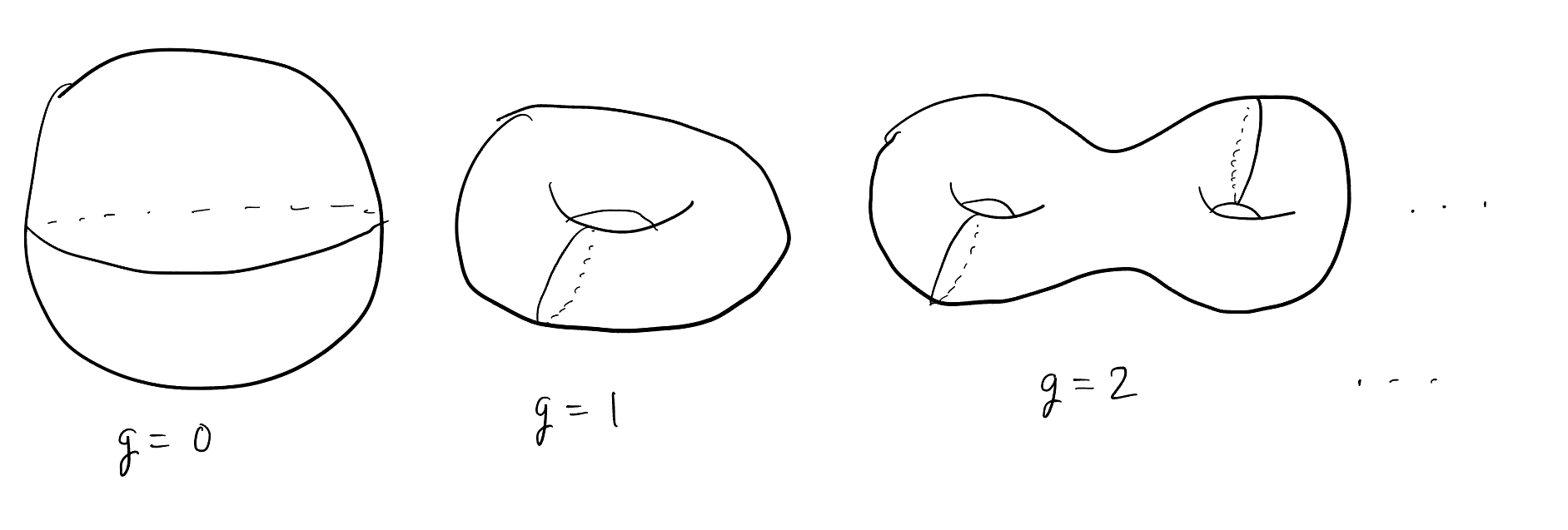
So when one computes a fairly abstract invariant, namely arithmetic genus, of a compact, connected complex curve, one is really just identifying which of the surfaces, depicted in the (infinitely long) list above, the complex curve looks like. Now we work toward actually computing the arithmetic genus.

The Hilbert Polynomial

The main point of this section is to define a polynomial invariant of coherent sheaves on projective $k$-schemes. This polynomial will be closely related to the arithmetic genus of the scheme and will allow us to compute the arithmetic genus of degree $d$ curves in the projective plane $\mathbb{P}_k^2$. We closely follow the construction/proof described in Theorem 18.6.1 of Vakil. First, we need to establish a theorem.

Lemma 3: Let $k$ be an infinite field. For any finite set of points $S\subseteq\mathbb{P}_k^n$, there exists a hyperplane that does not intersect $S$.

Proof: Let $S=\{p_1,\dots,p_m\}$. We will induct on $m$. Write $p_i=[p_i^0,p_i^1,\dots,p_i^n]$ for each $i$. Note that for each $i$, there exists at least one $j$ for which $p_i^j\neq0$. The case of $m=1$ is easy: pick $j$ for which $a_1^j\neq0$, and then the hyperplane cut out by $x_j$ does not contain $p_1$.

Now suppose that the hyperplane cut out by $\sum_{\ell=0}^{n}{a_{\ell}x_{\ell}}=0$ does not intersect $S$ and let $p_{m+1}$ be a point distinct from all points in $S$. Let $j$ be chosen so that $p_{m+1}^j\neq0$ and define $T=\{1\leq i\leq m+1\colon p_i^j\neq0\}$. Now observe that since $k$ is infinite and $T$ is finite, we may choose a $\lambda\in k$ such that

for any $i\in T$. Then by construction, the hyperplane cut out by

avoids $\{p_1,p_2,\dots,p_{m+1}\}$. This completes the induction. $\square$

Theorem 4: Let $k$ be an infinite field and let $X$ be a projective $k$-scheme. Suppose $\mathcal{F}$ is a coherent sheaf on $X$ and $\mathcal{L}$ is a very ample invertible sheaf on $X$. Then there exists an effective Cartier divisor $D$ on $X$, that does not contain the associated points, with $\mathcal{L}\cong\mathcal{O}(D)$.

Proof: Since $\mathcal{L}$ is very ample, there exist global sections $s_0,s_1,\dots,s_n$ of $\mathcal{L}$, with no common zeros, inducing a closed embedding $\pi\colon X\hookrightarrow\mathbb{P}_k^n$. Finitely generated modules over Noetherian rings have finitely many associated prime ideals (Vakil 6.6.17), so the coherent sheaf $\mathcal{F}$ has finitely many associated points. By Lemma 3 above, we can find a hyperplane $H\subseteq\mathbb{P}_k^n$ that avoids the image under $\pi$ of these points.

Note that by construction, $\mathcal{L}\cong\pi^{*}(\mathcal{O}_{\mathbb{P}_k^n}(1))$. So if $h$ is the section of $\mathcal{O}_{\mathbb{P}_k^n}(1)$ cutting out the hyperplane $H$, the pullback $\pi^{*}(h)$ can be identified with a global section $s$ of $\mathcal{L}$. The vanishing locus of this section avoids all of the associated points of $P$ since $H$ avoids the image of the associated points. Therefore, by Exercise 15.6.D of Vakil, the vanishing locus of $s$ cuts out an effective Cartier divisor $D$, and $\mathcal{L}\cong\mathcal{O}(D)$. $\square$

Now we can state the main definition of this section, though to check that the definition is well-formed, we will need to use Theorem 4 above.

Definition 3/Theorem 5: Let $\mathcal{F}$ be a coherent sheaf on a projective $k$-scheme $X\hookrightarrow\mathbb{P}_k^n$. The Euler characteristic $\chi(X,\mathcal{F}(m))$ is polynomial in $m$, and the degree of this polynomial is $\dim{\operatorname{Supp}{\mathcal{F}}}$. This polynomial is called the Hilbert polynomial of $\mathcal{F}$.

Proof: First, consider the case that $\mathcal{F}$ is the zero sheaf: all of the Betti numbers of the twists are zero, so the Euler characteristic is the constant zero polynomial. Now we specialize to the case that $\mathcal{F}$ is not the zero sheaf.

We induct on $\dim{\operatorname{Supp}{\mathcal{F}}}$. Note that cohomology respects base change (Exercise 18.2.H of Vakil) so we may assume without loss of generality that $k$ is an infinite field. Now we may take $\mathcal{L}=\mathcal{O}_X(1)$ in Theorem 4 above. The theorem then tells us that there exists a hyperplane $D$ that is the vanishing of the global section $s\in\Gamma(X,\mathcal{O}_X(1))$. Moreover, $D$ avoids all of the associated points of $\mathcal{F}$.

First if $\dim{\operatorname{Supp}{\mathcal{F}}}=0$, the support of $\mathcal{F}$ must be some finite set of closed points $x_1,x_2,\dots,x_{\ell}$ (see Vakil Exercise 12.1.C). Therefore, $\mathcal{F}$ is a finite direct sum of skyscraper sheaves, with each summand supported at exactly one of the $x_i$. Note that skyscraper sheaves are flabby since we may extend every section to a global section by just choosing a fixed value in the support and zero elsewhere. Therefore, the higher cohomology of skyscraper sheaves vanish, so the only nontrivial Betti number is $h^0$. Since cohomology commutes with colimits, it follows that the same is true of $\mathcal{F}$. Twisting does not change the stalks, so we conclude that $\chi(X,\mathcal{F}(m))=h^0(X,\mathcal{F})$, which is a constant polynomial in $m$.

Now suppose that $\mathcal{F}$ is a nonzero sheaf and coherent sheaves with lower dimensional supports than $\mathcal{F}$ have Hilbert polynomials. Note that $\mathcal{F}$ and $\mathcal{F}(-1)$ are both $\mathcal{O}_X$-modules. Moreover, they are both locally free sheaves of the same rank, so they have isomorphic stalks. Their stalks $\mathcal{F}_x\cong\mathcal{F}(-1)_x$ are $\mathcal{O}_{X,x}$-modules, and we have constructed $s$ in such a way that $s$ does not vanish at any associated point of $M$. Therefore by Proposition 6.6.13 of Vakil, the germ of $s$ is not a zero divisor for $\mathcal{F}_x\cong\mathcal{F}(-1)_x$ at any point $x\in X$. Hence the morphism $\mu_s\colon\mathcal{F}(-1)\to\mathcal{F}$ induced by multiplication by $s$ is a monomorphism of sheaves and we have a short exact sequence

Note that $\operatorname{coker}{\mu_s}$ is a coherent sheaf (since the category of coherent sheaves is Abelian). Now it follows from a fact in commutative algebra (Vakil Exercise 6.6.D) that $\operatorname{Supp}{\operatorname{coker}{\mu_s}}=(\operatorname{Supp}{\mathcal{F}})\cap D$. By Exercise 12.3.D(a) of Vakil, $V(x)$ meets every irreducible component of $\operatorname{Supp}{\mathcal{F}}$ of positive dimension. In particular, it meets an irreducible component of maximal dimension. Since $\mathcal{F}$ is nonzero, by Krull’s principal ideal theorem, the codimension of the intersection of $V(x)$ in every irreducible component of $\operatorname{Supp}{\mathcal{F}}$ is equal to $1$. Since this is true in particular in an irreducible component of $\operatorname{Supp}{\mathcal{F}}$ of maximal dimension, it follows that $\dim{\operatorname{Supp}{\operatorname{coker}{\mu_s}}}=\dim{\operatorname{Supp}{\mathcal{F}}}-1$.

$\mathcal{O}_X(m)$ is a locally free sheaf, so tensoring with it will preserve exactness. Hence for any $m$, we may twist the short exact sequence above to obtain

Euler characteristic is additive on exact sequences so for all $m$, we have

By the inductive hypothesis, the right hand side of the above equation is a polynomial in $m$ of degree $\dim{\operatorname{Supp}{\operatorname{coker}{\mu_s}}}=\dim{\operatorname{Supp}{\mathcal{F}}}-1$. Now it is a combinatorial exercise in finite differences that the above identity implies that $\chi(X,\mathcal{F}(m))$ is a polynomial in $m$ of degree $\dim{\operatorname{Supp}{\mathcal{F}}}$. This completes the induction. $\square$

For $\mathcal{F}=\mathcal{O}_X$, this polynomial is often called the Hilbert polynomial of $X$, which we will denote by $p_X(m)$. Observe that by definition, the constant term of the Hilbert polynomial is closely related to the arithmetic genus: $p_X(0)=1+(-1)^np_a(X)$. Note that by the Serre vanishing theorem, we have $\chi(X,\mathcal{F}(m))=h^0(X,\mathcal{F}(m))$ for $m$ sufficiently large.

These facts give us the historical point of view. The Hilbert polynomial was first obtained by calculating the number of independent degree $m$ functions on $X$, which is the Betti number $h^0(X,\mathcal{O}_X(m))$. The observation was that for large $m$ these numbers fit a polynomial, and that when $X$ is a curve the constant term of this polynomial was effectively the topological genus of the curve! This is probably the closest thing to magic one can experience with just paper and pen.

We now calculate the Hilbert polynomial in some nice cases. Note that for $m\geq0$, $h^0(\mathbb{P}_k^n,\mathcal{O}(m))$ counts the number of degree $m$ monomials in $n$ variables. Hence by Serre vanishing, we have

In particular, $p_a(\mathbb{P}_k^n)=(-1)^n\left(\binom{n}{n}-1\right)=0$, which is very reasonable! Now we can calculate the Hilbert polynomial which will give us the genus of the Fermat curve.

Theorem 6: The Hilbert polynomial of a degree $d$ hypersurface $H$ in $\mathbb{P}_k^n$ is

Proof: Let $\iota\colon H\hookrightarrow\mathbb{P}_k^n$ be the closed embedding. If $H$ is cut out by the degree $d$ function $f\in\mathcal{O}_{\mathbb{P}_k^n}(d)$, multiplication by $f$ induces the short exact sequence for the closed embedding:

Hence by the additivity of Euler characteristic, it follows that

$\square$

Corollary: The arithmetic genus of a degree $n$ curve in the projective plane is

Hence by Theorem 3, the geometric genus of the Fermat curve $F_k^n$ is as above as well.

The Riemann–Roch Theorem

We have been making extensive use of cohomological techniques so far, and we will continue with another result about divisors on curves, namely the Riemann–Roch theorem. Since Weil divisors on a curve are (roughly) in correspondence with line bundles on the curve, this result can alternatively be thought of as a result about the cohomology of line bundles on a curve. Serre duality will continue to be a crucial technical tool in this discussion.

In this discussion, by “curve” we mean an integral, separated, $1$-dimensional smooth scheme of finite type and proper over a field $k$. Note that in particular, the condition of being proper over a field $k$ implies that our curves are projective (Proposition II.6.7 of Hartshorne).

Definition 4: Let $X$ be a curve over a field $k$, with structure morphism $\varphi\colon X\to\operatorname{Spec}{k}$. Let $S$ be a finite set of dimension $0$ points of $X$, and for each $p\in S$ let $\varphi_p^{\sharp}\colon k\hookrightarrow k(p)$ be the extension of residue fields induced by $\varphi$. Let $D=\sum_{p\in S}{a_pp}$ be a divisor. Then we define the degree of $D$ to be

Notice that in the case that $k$ is algebraically closed, it follows from Exercise 5.3.F of Vakil that $k(p)\cong k$, and thus the degree of $D$ becomes the more familiar quantity $\sum_{p\in S}{a_p}$. This more general notion of degree will allow us to state a version of the Riemann–Roch theorem that works over arbitrary fields.

Theorem 7 (Riemann–Roch): Let $X$ be a curve over any field $k$ and let $D$ be a divisor on $X$. Then

Proof: Write $D=\sum_{p\in S}{a_pp}$. We induct on $\sum_{p\in S}{|a_p|}$. In the base case, we have $D=0$. In this case, $\mathcal{O}(D)\cong\mathcal{O}_X$, so the conclusion is immediate.

Now suppose the claim is true for some divisor $D$. Pick a (closed) point $p\in X$. Then $p$ is a closed subscheme of $X$ and thus gives the closed subscheme short exact sequence

Note that $\mathcal{O}_X|_p$ is simply a skyscraper sheaf of the residue field $k(p)$. So when we tensor the about exact sequence by the rank \(1\) locally free sheaf $\mathcal{O}(D+p)$, this skyscraper sheaf will be preserved. Hence we have

Now since Euler characteristic is additive on exact sequences, we have

with the last equality following from the inductive hypothesis. But we can explicitly compute the Euler characteristic of $\mathcal{O}_X|_p$ since we know it is just a skyscraper sheaf which is flabby. We have

This completes the induction. $\square$

The Riemann–Roch theorem is often written in various different ways. For example, we may observe that since since $X$ is projective, Serre duality applies and says $H^1(X,\mathcal{O}(D))\cong H^0(X,\omega_X\otimes\mathcal{O}(-D))^*$. Moreover, $\chi(X,\mathcal{O}_X)=1-p_a(X)$. So the Riemann–Roch theorem states

where $K_X$ is the canonical divisor of $X$. The useful consequence of this for us will be what results from letting $D=K_X$. Then we obtain

and after an application of Theorem 3, we have the following formula for the degree of the canonical divisor.

Corollary: For a curve $X$, the degree of the canonical divisor is

We will need this formula to prove the Riemann–Hurwitz theorem.

Ramification

We now discuss the important geometric concept of ramification. We continue to use the same definition of “curve” as in the section above.

Let $X$ be a locally Noetherian scheme. Consider a regular codimension $1$ point $p\in X$. The stalk $\mathcal{O}_{X,p}$ at such a point is a regular local ring of dimension $1$. It is now a fact from commutative algebra that the stalk $\mathcal{O}_{X,p}$ must be a discrete valuation ring.

Definition 5: Let $\pi\colon X\to Y$ be a finite morphism of curves over any field. Let $p\in X$ be a point, let $\pi^{\sharp}\colon\mathcal{O}_{Y,\pi(p)}\to\mathcal{O}_{X,p}$ be the induced map on stalks, and let $t$ be a uniformizing parameter of the DVR $\mathcal{O}_{Y,\pi(p)}$. We define the ramification index of $\pi$ at $p$, denoted $e_p$, to be the valuation of $\pi^{\sharp}(t)$.

We also adopt some obvious terminology, such as ramification locus for the set of points $p$ for which $e_p>1$, branch points for the points that are in the image of the ramification locus, and so on. In order to geometrically understand the ramification and branch loci, we need to develop the following lemma.

Note that if $X$ and $Y$ are nonsingular varieties over a field $k$, and $\pi\colon X\to Y$ is a nonconstant finite morphism, Proposition II.6.7 and II.6.8 of Hartshorne imply that $\pi$ is surjective (and hence, dominant). It follows that there is an induced extension of function fields $K(Y)\hookrightarrow K(X)$. The degree of $\pi$ is defined to be the degree of this field extension. We say that $\pi$ is separable if the induced field extension is separable.

Lemma 4: Let $\pi\colon X\to Y$ be a finite separable morphism of irreducible varieties of the same dimension $n$ over a field $k$. Let $Y$ be smooth. Then there exists a short exact sequence of sheaves on $X$:

Proof: Since $\pi$ is a morphism of $k$-schemes, we already have the relative cotangent sequence

Since $Y$ is smooth, $\Omega_{Y/k}$ is a locally free sheaf of rank $n$ on $Y$, and thus $\pi^{*}(\Omega_{Y/k})$ is a locally free sheaf of rank $n$ on $X$. Since localizations of torsion-free modules are themselves torsion-free, it follows that $\pi^{*}(\Omega_{Y/k})$ is a torsion-free sheaf.

Note that if $M$ is a torsion-free module over an integral domain $A$, then if the localization of $M$ at the zero ideal vanishes, we must have $M=0$. Therefore to show that $\phi$ is injective, it suffices to show that the stalk of the subsheaf $\ker{\phi}$ of $\pi^*(\Omega_{Y/k})$ at the generic point of $X$ is zero.

Let $\eta$ be the generic point of $X$. Stalkification is an exact functor, so we have the exact sequence

Since $\Omega_{Y/k}$ and $\pi^{*}(\Omega_{Y/k})$ both locally free of rank $n$, their stalks are isomorphic to $\mathcal{O}_{X,\eta}^{\oplus n}$. Meanwhile, by Proposition II.8.2A of Hartshorne, localization commutes with taking modules of Kähler differentials, so we have $(\Omega_{X/Y})_{\eta}\cong\Omega_{K(X)/K(Y)}$. But $K(Y)\hookrightarrow K(X)$ is a separable field extension, so for every $\alpha\in K(X)$, there exists a polynomial $f(t)\in (K(Y))[t]$ such that $f(\alpha)=0$ and $f’(\alpha)\neq0$. In particular, $f’(\alpha)\, d\alpha=0$ so $d\alpha=0$, hence $(\Omega_{X/Y})_{\eta}\cong 0$. Therefore, the above exact sequence becomes

In particular, $\phi_{\eta}$ is a surjection between free modules (in fact, vector spaces) of the same (finite) rank, so $\phi_{\eta}$ is an injection. $\square$

This lemma will allow us to say much more about ramification. As a first result, we can establish that in the reasonable cases, ramification only occurs finitely often.

Theorem 8: Let $\pi\colon X\to Y$ be a finite separable morphism of curves. Then $\pi$ is ramified at only finitely many points.

Proof: Let $p\in X$ be a point and let $u$ be a uniformizing parameter of the DVR $\mathcal{O}_{X,p}$ and $t$ a parameter for $\mathcal{O}_{Y,\pi(p)}$. Then the differential $dt$ generates $(\Omega_{Y/k})_{\pi(p)}$ as a $\mathcal{O}_{Y,\pi(p)}$-module and $du$ generates $(\Omega_{X/k})_{p}$ as a $\mathcal{O}_{X,p}$-module by II.8.7 and II.8.8 of Hartshorne. Then, $\pi^{*}(dt)$ generates $\pi^{*}(\Omega_{Y/k})_p$.

By exactness, the stalk $(\Omega_{X/Y})_p$ vanishes precisely when the map on stalks $\phi_p$ is surjective, where $\phi\colon \pi^{*}(\Omega_{Y/k})\to\Omega_{X/k}$ is the map of sheaves in the short exact sequence from Lemma 4. This occurs if and only if $\phi_p(\pi^{*}(dt))$ is a generator of $(\Omega_{X/k})_p$. Since $u$ is a uniformizing parameter for $\mathcal{O}_{X,p}$, we may write $\pi^{\sharp}(t)=su^e$ for some unit $s\in\mathcal{O}_{X,p}$ and nonnegative integer $e$. Hence, we may write

Here of course we interpret $e$ as the sum of $1$ with itself $e$ times in the ring $\mathcal{O}_{X,p}$. Since $du$ generates $(\Omega_{X/k})_p$, we can write $ds=h\, du$ for some $h\in\mathcal{O}_{X,p}$. Hence, the above equation becomes

If the characteristic of $k$ divides $e$, then the above becomes $hu^e\, du$, where $hu^e$ is in the maximal ideal $\langle u\rangle$ and thus not a unit. Hence, $\phi_p$ will not be surjective in this case.

On the other hand, if the characteristic of $k$ does not divide $e$, then $e\neq0$. Note also that since $X$ is a $k$-scheme, we may interpret $e$ as the germ of a nonzero constant function at $p$, so it is a unit in $\mathcal{O}_{X,p}$. Therefore, $hu+es$ is the sum of an element of the maximal ideal with a unit in a local ring, and thus is a unit. Therefore, in the case that $e\neq0$, we note that $\phi_p$ is surjective if and only if $e=1$.

Hence we have shown that $\phi_p$ is surjective (so $(\Omega_{X/Y})_p=0$) if and only if $\pi$ unramified at $p$. That is, the ramification locus of $\pi$ is precisely the support of $\Omega_{X/Y}$. In the proof of Lemma 4, we showed that $\Omega_{X/Y}$ is a torsion sheaf (its stalk at the generic point is zero). It follows (by Exercise 14.3.F(b) of Vakil) that the support of $\Omega_{X/Y}$ lies in the complement of a dense open subset of $X$. That is, the ramification locus of $\pi$ lies in a finite set. $\square$

With Theorem 8 in hand, it now makes sense to make the following definition. We denote the length of a module $M$ by $\ell(M)$.

Definition 6: Let $\pi\colon X\to Y$ be a finite separable morphism of curves. We define the ramification divisor of $\pi$, denoted $R_{\pi}$ to be the divisor $\sum_{p\in X}{\ell((\Omega_{X/Y})_p)p}$, and we define the branch divisor of $\pi$, denoted $B_{\pi}$, to be $\pi_{*}(R_{\pi})$.

The proof of Theorem 8 also shows us that there are two kinds of ramification, and they behave somewhat differently on an algebraic level.

Definition 7: Let $\pi\colon X\to Y$ be a finite morphism of curves over the field $k$. Suppose $\pi$ is ramified at $p\in X$. If the characteristic of $k$ is zero or does not divide $e_p$, we say that the ramification of $\pi$ at $p$ is tame. Otherwise, we say that the ramification of $\pi$ at $p$ is wild.

We have already seen from the proof of Theorem 8 that $\pi$ is unramified at $p$ if and only if $\ell((\Omega_{X/Y})_p)=0$. This is why Definition 5 makes sense: it forces the formal sum in the definition of the ramification divisor to be a finite sum. So the length of the stalk of $\Omega_{X/Y}$ is a measure of the “amount” of ramification occurring at the point. However, it turns out that there is a quantitative difference between how tame and wild ramification are related to the length of the stalk.

Theorem 9: Let $\pi\colon X\to Y$ be a finite separable morphism of curves and let $p\in X$ be a point. Then

with equality occuring if and only if $\pi$ is unramified at at $p$ (which occurs precisely when $e_p=1$), or if $\pi$ is tamely ramified at $p$.

Proof: We will use the notation from the proof of Theorem 8. Since $\pi^{*}(dt)$ generates $\pi^{*}(\Omega_{Y/k})_p$, there exists a unique element $g\in\mathcal{O}_{X,p}$ such that $\phi_p(\pi^{*}(dt))=g\, du$, where $\phi\colon \pi^{*}(\Omega_{Y/k})\to\Omega_{X/k}$ is the map of sheaves in the short exact sequence from Lemma 4. More generally, we may write

for any $h\in\mathcal{O}_{X,p}$. This characterizes the map $\phi$. Hence by Lemma 4, we have the isomorphism of $\mathcal{O}_{X,p}$-modules $(\Omega_{X/Y})_p\cong\operatorname{coker}{\phi_p}\cong\mathcal{O}_{X,p}/\langle g\rangle$. Thus,

where $v(g)$ is the valuation of $g$. The last equality is a fact of commutative algebra and essentially follows from the pigeonhole principle: a chain of submodules of $\mathcal{O}_{X,p}$ containing $g$, with length larger than $v(g)$, must contain repeated submodules since every element of $\mathcal{O}_{X,p}$ is uniquely expressed as $su^k$ where $s$ is a unit.

Now, recall that we computed in the proof of Theorem 8 that

where $s$ is a unit in $\mathcal{O}_{X,p}$ and $e=e_p$ is the ramification index of $\pi$ at $p$. As we observed in the proof of Theorem 8, if $\pi$ is wildly ramified at $p$, this expression reduces to $hu^e\, du$, where $hu^e$ is not a unit, and thus $v(g)=v(hu^e)\geq e>e-1$. If $\pi$ is tamely ramified at $p$, we saw that $hu+es$ is a unit, and thus $v(g)=v((hu+es)u^{e-1})=e-1$. Finally, we saw in the proof of Theorem 8 that $\pi$ is unramified at $p$ if and only if $e=1$. $\square$

Note that from a geometric point of view, only tame ramification is relevant since this is all that can occur in characteristic zero. So what exactly is so “geometric” about this concept of ramification? Recall that the fiber of a finite morphism between curves will be finite set. The following technical lemma is Exercise 16.3.D(b) of Vakil, which shows that the degree of the morphism consists of contributions from each element of the fiber over any closed point.

Lemma 5: Let $\pi\colon X\to Y$ be a nonconstant finite morphism of curves and let $q\in Y$ be a closed point. For each point $p\in\pi^{-1}(\{q\})$, let $\overline{\pi}_p^{\sharp}\colon k(q)\hookrightarrow k(p)$ be the induced extension of residue fields. Then

Proof: First, we call upon Proposition 16.3.5 of Vakil. $\pi$ is dominant, so it takes the generic point of $X$ to the generic point of $Y$. Since $\pi_*(\mathcal{O}_X)$ is locally free and stalkification is exact, it follows that the rank of $\pi_*(\mathcal{O}_X)$ will equal the rank of the stalk $K(X)$ with respect to the $K(Y)$-module structure induced by the map on stalks at the generic points $\pi_{\eta}^{\sharp}\colon K(Y)\hookrightarrow K(X)$. That is, Hartshorne’s definition of degree of a map (which is what we use) agrees with Vakil’s: $\deg{\pi}=\operatorname{rank}{\pi_*(\mathcal{O}_X)}$.

Next, we need to observe that immediately from the definitions, we have the decomposition of the $\mathcal{O}_{Y,q}$-module $(\pi_*(\mathcal{O}_X))_q$ given by

and thus it suffices to show that for a fixed choice of $p\in \pi^{-1}(\{q\})$, we have $\operatorname{rank}_{\mathcal{O}_{Y,q}}{\mathcal{O}_{X,p}}=e_p[k(p):\overline{\pi}_p^{\sharp}(k(q))]$.

Fix such a point $p$ and let $u_p$ be a uniformizing parameter of the DVR $\mathcal{O}_{X,p}$, and let $t$ be a parameter for $\mathcal{O}_{Y,q}$. Let us abbreviate $d_p:=[k(p):\overline{\pi}_p^{\sharp}(k(q))]$ and let $\overline{w_{p,1}},\overline{w_{p,2}},\dots,\overline{w_{p,d_p}}$ be a $k(q)$-basis for $k(p)$. The maximal ideal of $\mathcal{O}_{X,p}$ is generated by $u_p$, so we may choose lifts $w_{p,i}\in\mathcal{O}_{X,p}$ of these basis elements whose valuations are zero (meaning they are units in $\mathcal{O}_{X,p}$). Now it follows quickly by construction that the set of elements of the form $w_{p,i}u_p^{j}$, for $i\in\{1,2,\dots,d_p\}$ and $j\in\{0,1,\dots,e_p-1\}$, is a linearly independent $\mathcal{O}_{Y,q}$-generating set of $\mathcal{O}_{X,p}$. Therefore, $\operatorname{rank}_{\mathcal{O}_{Y,q}}{\mathcal{O}_{X,p}}=e_pd_p$ as claimed. $\square$

Theorem 10: Let $\pi\colon X\to Y$ be a finite morphism of curves over an algebraically closed field $k$. Let $q\in Y$ be chosen so that the ramification of $\pi$ at every point in the fiber $\pi^{-1}(\{q\})$ is tame. Then,

Proof: Since $q$ is a closed point and $p$ is a closed point for every $p$ in the fiber over $q$, it follows (Exercise 5.3.F of Vakil) that both $k(p)$ and $k(q)$ are finite (and thus, algebraic) extensions of $k$. But $k$ is algebraically closed, so $k(p)\cong k(q)\cong k$ and thus in the notation of Lemma 5, $d_p=1$ for all $p\in \pi^{-1}(\{q\})$. Therefore, Lemma 5 and Theorem 8 yield

$\square$

This finally gives us a geometric interpretation of ramification (at least in characteristic zero where all ramification is tame). Generically, the size of the fibers of $\pi$ is $\deg{\pi}$. However, over branch points, the number is smaller. Hence we may interpret $\pi$ as a sort of generically $(\deg{\pi})$-sheeted cover, with ramification points just being places where these sheets collide.

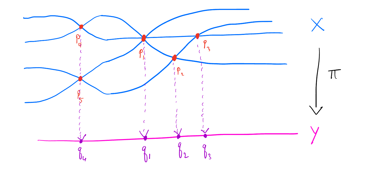
In the depiction of tame ramification over an algebraically closed field above, $\deg{\pi}=4$ which is the size of the generic fiber, the ramification divisor is $R_{\pi}=2p_1+p_2+p_3+p_4+p_5$, the branch divisor is $B_{\pi}=2q_1+q_2+q_3+2q_4$, and we can see that the formula for the size of the fibers from Theorem 10 holds true. In general, we see that the ramification index at any point in $X$ measures precisely the number of sheets passing through that point. A canonical example of this would be the map $z\mapsto z^2$ on the complex plane to itself. Every nonzero complex number has two square roots, but the map is ramified at zero. See here for some nice visuals of Riemann surfaces arising as graphs of algebraic functions from the complex plane to itself.

The Riemann–Hurwitz Formula

We can finally state and prove the main result.

Theorem 11 (Riemann–Hurwitz): Let $\pi\colon X\to Y$ be a finite separable morphism of curves. Then

Proof: We start by considering the ramification divisor $R_{\pi}$ as a closed subscheme of $X$. Let $\iota\colon R_{\pi}\to X$ be the closed embedding. This gives the short exact sequence

Taking determinants in this exact sequence, we find that $\mathcal{O}_X(-R_{\pi})\otimes\det{\iota_{*}(\mathcal{O}_{R_{\pi}})}\cong\mathcal{O}_X$, which means $\det{\iota_{*}(\mathcal{O}_{R_{\pi}})}\cong\mathcal{O}_X(R_{\pi})$. We also see from the proof of Theorem 8 that the structure sheaf of $R_{\pi}$ is isomorphic to the restriction of $\Omega_{X/Y}$ to $R_{\pi}$. Since $R_{\pi}$ is the support of $\Omega_{X/Y}$, we have that

hence we have shown that $\det{\Omega_{X/Y}}\cong\mathcal{O}_X(R_{\pi})$. Now we can take determinants in the short exact sequence of Lemma 4. This gives

For a finite morphism of curves $\pi$, determinant will commute with pullback. Hence the above completely simplifies to $\pi^*(\omega_Y)\otimes\mathcal{O}_X(R_{\pi})\cong\omega_X$. Taking the associated divisors, we have the linear equivalence:

This is sometimes known as the strong Riemann–Hurwitz theorem. Our result follows from this by taking the degrees of both sides. By our corollary to the Riemann–Roch theorem, we know that $\deg{K_X}=2g(X)-2$ and $\deg{K_Y}=2g(Y)-2$. By Proposition II.6.9 of Hartshorne, the degree of the pullback is the product of the degree of the divisor with the degree of the map. Thus the formula follows. $\square$

So ultimately, given a reasonable map $\pi\colon X\to Y$ of curves, the genera of the curves $X$ and $Y$ must be related to the degree and ramification of $\pi$.

A nonconstant morphism between curves (under our definition of “curve”) must be finite by Proposition II.6.8 of Hartshorne. Moreover, in characteristic $0$, every finite morphism is automatically separable since the formal derivative of any nonzero nonconstant polynomial will be nonzero. Therefore, we are now in a position to extend Theorem 1 to the setting of any base field $k$ of characteristic $0$.

Proof 2 of Theorem 1: Suppose that $k$ is a field of characteristic $0$ and $\pi\colon\mathbb{P}^1_k\dashrightarrow F_k^n$ is a dominant rational map. By the curve-to-projective extension theorem, this promotes to a genuine finite morphism $\tilde{\pi}\colon \mathbb{P}^1_k\to F_k^n$. Moreover, this morphism is separable since $k$ has characteristic $0$. Hence, the Riemann–Hurwitz theorem tells us that

By Theorem 2, Theorem 3, and the corollary to Theorem 6, we can fill out the genera of the two curves, so the above equation becomes

But $n\geq 3$, so $(n-1)(n-2)-2\geq0$. Moreover, $\deg{\tilde{\pi}}\geq1$ and $\deg{R_{\tilde{\pi}}}\geq0$. Therefore the right hand side of the equation above should be nonnegative, a contradiction. $\square$

Parameterized Rational Solution Sets

Now that we have thoroughly discussed Theorem 1, let us discuss its relationship with Fermat’s last theorem. Classically, we are interested in integer (or equivalently, rational) solutions to the equation $x^n+y^n=z^n$ for $n>2$. When $n=2$, the problem is very simple. There are infinitely many solutions to the equation, and they are the Pythagorean triples. In fact, the entire infinite family of solutions can be parameterized by the projective line as follows.

Theorem 12: Let $k$ be a field of characteristic not equal to $2$. Then the conic $x^2+y^2=z^2$ in $\mathbb{P}^2_k$ is isomorphic to the projective line $\mathbb{P}^1_k$.

Proof: Let $C$ be the conic. Note that $[-1,0,1],[1,0,1]\in C$. Put $U=C\setminus\{[-1,0,1]\}$ and $V=C\setminus\{[1,0,1]\}$. Let us define a map $\psi_U\colon U\to\mathbb{P}^1_k$ by $\psi_U([x,y,z])=[x+z,y]$. Note that this is well-defined by the definition of $U$—it will never be the case that both $y$ and $x+z$ vanish on $U$. Similarly, we may define a map $\psi_V\colon V\to\mathbb{P}^1_k$ by $\psi_V([x,y,z])=[y,z-x]$. Of course, on the overlap $U\cap V$, we may note that since $y^2=(x+z)(z-x)$, we have that $\psi_U|_{U\cap V}=\psi_V|_{U\cap V}$. So $\psi_U$ and $\psi_V$ glue to a morphism $\psi\colon C\to\mathbb{P}^1_k$.

An inverse map $\varphi\colon\mathbb{P}^1_k\to C$ can be defined by $\varphi([x,y])=[x^2-y^2,2xy,x^2+y^2]$. Note then that if $x\neq0$, we have $[2x^2,2xy]=[x,y]$ and if $y\neq0$, we have $[2xy,2y^2]=[x,y]$. Hence, $\psi\circ\varphi$ is the identity. For similar reasons, we can see that $\varphi\circ\psi$ is the identity. Note that this argument works as long as $2\neq0$, which occurs as long as $k$ does not have characteristic 2. $\square$

The isomorphism given in the theorem above yields a parameterization of all rational Pythagorean triples. Select $k=\mathbb{Q}$ above. Then by the isomorphism above, any Pythagorean triple $a,b,c$ must form a point in projective space $[a,b,c]$ equal to $[x^2-y^2,2xy,x^2+y^2]$ for some choice of point $[x,y]\in\mathbb{P}_{\mathbb{Q}}^1$. In particular, by scaling the homogeneous coordinates and clearing the denominators, we may assume without loss of generality that $x$ and $y$ are integers. By scaling and factoring out the greatest common divisor, we may also assume that $x$ and $y$ are coprime. Then, we have

where $\lambda$ is a rational number, say $\frac{p}{q}$ for coprime integers $p$ and $q$. This alone is good enough, but lets push this further to something you would encounter classically.

Since $b=2\lambda xy$ is an integer, we must have $q\mid 2xy$. Let $s$ be a prime factor of $q$. If $s\mid y$, we have that $s\mid y^2$, so that $s\mid x^2$, since $c=x^2+y^2$ is an integer. So $s\mid x$, violating our assumption that $x$ and $y$ are coprime. Hence, $s\nmid y$, and similarly $s\nmid x$. It follows that $s=2$, so $q$ is a power of $2$.

Suppose that $x$ and $y$ are not both odd. Then since they are coprime, one of them is odd and the other is even. Therefore, $x^2+y^2$ is odd. But $c=\lambda(x^2+y^2)$ must be an integer and $q$ is a power of $2$. Hence we must have $q=1$ in this situation, so $\lambda$ can be taken to be an integer.

If $x$ and $y$ are both odd, then $a$, $b$, and $c$ are even. This means that we can write $a=2^i\alpha$, $b=2^j\beta$, and $c=2^k\gamma$, for odd numbers $\alpha$, $\beta$, and $\gamma$, and positive integers $i$, $j$, and $k$. Note that

Without loss of generality, suppose $i\leq j$. It is impossible for $k<i$, since if this were the case, dividing both sides of the above equation by $2^{2k}$, the above equation would have an even left hand side but an odd right hand side. Hence, when we divide the above equation by $2^{2i}$ to obtain

we have obtained the Pythagorean triple $\alpha$, $2^{j-i}\beta$, and $2^{k-i}\gamma$. Note that we must have $j-i>0$, since otherwise we have a Pythagorean triple where both summands are odd, which is impossible as is seen by reducing the Pythagorean equation modulo $4$. Hence, $2^{j-i}\beta$ is genuinely even. This new Pythagorean triple is obtained by some homogeneous coordinate $[\tilde{x},\tilde{y}]$ where $\tilde{x}$ and $\tilde{y}$ are coprime integers. We may write

where $\tilde{\lambda}$ is a rational number. By our past argument a few paragraphs above, we know that the denominator $\tilde{q}$ of $\tilde{\lambda}$ must be a power of $2$. Suppose $\tilde{x}$ and $\tilde{y}$ are both odd. Since $2^{j-i}\beta=2\tilde{\lambda}\tilde{x}\tilde{y}$ needs to be an integer, it follows that $\tilde{q}=2$ or $\tilde{q}=1$ are the only positive choices for $\tilde{q}$. If $\tilde{q}=2$, since $\tilde{x}^2-\tilde{y}^2$ must be a multiple of $4$, it follows that $\alpha=\tilde{\lambda}(\tilde{x}^2-\tilde{y}^2)$ is a multiple of $2$, a contradiction. Therefore, $\tilde{q}=1$ if $\tilde{x}$ and $\tilde{y}$ are both odd, so $\tilde{\lambda}$ can be taken to be an integer. If $\tilde{x}$ and $\tilde{y}$ are not both odd, by our past argument a few paragraphs above, it follows that $\tilde{q}=1$. Hence, $\tilde{\lambda}$ can be taken to be an integer in every case.

Hence in the case that $x$ and $y$ are both odd, we can replace $x$ and $y$ with integers $\tilde{x}$ and $\tilde{y}$ that are not both odd, and then select $\lambda$ to be an integer: $\lambda=2^i\tilde{\lambda}$.

To sum up, we have shown that $x$ and $y$ can be judiciously chosen so that $\lambda$ can always be taken to be an integer, and that these $x$ and $y$ can be chosen to not both be odd. That is, the Pythagorean triples are generated by the triples of the form

where $x$ and $y$ are coprime integers, not both odd, and $\lambda$ is an integer. This is the classical Euclid’s formula for generating Pythagorean triples, and it essentially falls out of the isomorphism between the conic $x^2+y^2=z^2$ and the projective line.

Theorem 1 establishes that at least over the complex numbers, there is no isomorphism between the projective line and the curve $x^n+y^n=z^n$ for $n>3$. Even though this is a statement over the complex numbers, by descent it has implications for the nature of rational solutions to the equation $x^n+y^n=z^n$ for $n>3$. Hence, the low brow proof shown above, which only works over $\mathbb{C}$, is sufficient for what follows about rational solutions.

The relevant result to show this is the following characterization of dominant morphisms.

Proposition 7.5.8 (Vakil)/Lemma 29.8.8 (Stacks): A morphism $f\colon X\to Y$ between integral $k$-schemes is dominant if and only if the induced map on stalks $\mathcal{O}_{Y,f(x)}\to\mathcal{O}_{X,x}$ is injective for any $x\in X$.

Fermat’s last theorem asserts that there are no rational solutions to $x^n+y^n=z^n$ for $n>2$. This is a far stronger statement than anything we have discussed which of course requires much more machinery. However, we have seen in the $n=2$ case that a dominant rational map from $\mathbb{P}^1_{\mathbb{Q}}$ to the Fermat curve over $\mathbb{Q}$ yields an infinite family of rational solutions to $x^n+y^n=z^n$ parameterized by the projective line.

Suppose such an infinite family of rational solutions exists for $n>3$. That is, suppose there exists a dominant rational map from $\mathbb{P}_{\mathbb{Q}}^1$ to the Fermat curve over $\mathbb{Q}$ for $n>2$. Let us denote the Fermat curve over $\mathbb{Q}$ as $F_{\mathbb{Q}}^{n}$. As we have seen with the curve-to-projective extension theorem, this extends to a dominant morphism $\phi_{\mathbb{Q}}\colon\mathbb{P}_{\mathbb{Q}}^1\to F_{\mathbb{Q}}^{n}$. By the Proposition/Lemma above, the induced morphism on function fields $\phi_{\mathbb{Q}}^{\sharp}\colon K(F_{\mathbb{Q}}^{n})\to K(\mathbb{P}_{\mathbb{Q}}^1)$ is injective.

Now we extend the base field to $\mathbb{C}$. Applying the change of base functor to the morphism $\phi_{\mathbb{Q}}$, we obtain the morphism $\phi_{\mathbb{C}}\colon\mathbb{P}_{\mathbb{C}}^1\to F_{\mathbb{C}}^1$. Looking at this new morphism on the stalks at the points corresponding to the generic points over $\mathbb{Q}$ amounts to performing an extension of scalars via the functor $-\otimes_{\mathbb{Q}}\mathbb{C}$ on the map $\phi_{\mathbb{Q}}^{\sharp}$. Since $\mathbb{Q}$ is a field, it is automatic that $\mathbb{C}$ is flat as a $\mathbb{Q}$-module since it is a vector space (free module). Therefore, the functor $-\otimes_{\mathbb{Q}}\mathbb{C}$ is exact and so the injectivity of $\phi_{\mathbb{Q}}^{\sharp}$ is preserved after base change. It follows from the Proposition/Lemma above, $\phi_{\mathbb{C}}$ is a dominant morphism. But such a thing cannot exist by Theorem 1.

So perhaps one moral of this story is that an extremely weak form of Fermat’s last theorem—that there is no $\mathbb{P}^1$-parameterized family of rational points on the Fermat curve for $n>2$—is true for entirely geometric reasons.

Making the identifications $H^0(X,\Omega_X^1)\cong H^{1,0}(X)$ and $H^1(X,\mathcal{O}_X)\cong H^{0,1}(X)$ so that the above decomposition looks more like the classical Hodge decomposition requires more, since the general fact $H^{p,q}(X)\cong H^q(X,\Omega_X^p)$, where $\Omega_X^p$ is the sheaf of holomorphic $p$-forms, requires some elliptic operator theory. We can also show that in our special case of a compact connected complex curve, $H^1(X,\mathcal{O}_X)\cong\overline{H^0(X,\Omega_X^1)}$, provided that we may assume that $H^1(X,\mathcal{O}_X)\cong H^{0,1}(X)$. Without this, we would have trouble interpreting the degree $1$ sheaf cohomology $H^1(X,\mathcal{O}_X)$. Theorems 4.49 and 4.50 of Voisin give some interpretations of sheaf cohomology in degree $1$. For example, using Čech cohomology, if $\mathcal{O}_X^{\times}$ is the sheaf of nonvanishing holomorphic functions on $X$, we can see that $H^1(X,\mathcal{O}_X^{\times})$ can be interpreted as the Picard group of $X$.

Note that any complex curve is automatically Kähler, since the real dimension is $2$ and so every $2$-form is immediately closed which makes any Hermitian metric on a complex curve Kähler. Therefore, a compact complex curve is a special case to which the Hodge decomposition should apply.

We start by fixing a compact connected complex curve $X$. In particular, we are dealing with a closed manifold, which is a compact manifold without boundary. This fact will be relevant for us later. Let $\mathcal{O}_X$ be the sheaf of holomorphic functions on $X$ and let $\Omega_X^1$ be the sheaf of holomorphic 1-forms. Since $X$ is a curve, any section of this sheaf can be expressed locally as simply $f\, \mathrm{d}z$ where $f$ is a holomorphic function and $z$ is a local coordinate.

The complex derivative of any holomorphic function is itself holomorphic, so exterior differentation furnishes a morphism of sheaves $d\colon\mathcal{O}_X\to\Omega_X^1$. From complex analysis (say, Cauchy’s theorem) we know that in simply connected neighborhoods, holomorphic functions have antiderivatives. This means that every section of $\Omega_X^1$ is at least locally exact. This is a special case of the more general Poincaré lemma. In any case, this means that $d$ is surjective on stalks—that is, it is an epimorphism of sheaves. Of course, the kernel of $d$ is the sheaf of locally constant functions $\underline{\mathbb{C}}$. Since $X$ is connected, this is the sheaf of constant functions. Hence we have a short exact sequence of sheaves: \[0\longrightarrow\underline{\mathbb{C}}\longrightarrow\mathcal{O}_X\xrightarrow[]{\,\, d\,\,}\Omega_X^1\longrightarrow0.\] This short exact sequence induces the following long exact sequence in sheaf cohomology:

We can fill out a few of modules in the above diagram.

1. Since $X$ is connected, we have $H^0(X,\underline{\mathbb{C}})\cong\mathbb{C}$.
2. Since $X$ is a compact Riemann surface, we have $H^0(X,\mathcal{O}_X)\cong\mathbb{C}$ by Liouville’s theorem.
3. $X$ is a complex curve, so its canonical bundle is just $\Omega_X^1$. Hence, by Serre duality \[H^1(X,\Omega_X^1)\cong H^0\left(X,(\Omega_X^1)^{*}\otimes \Omega_X^1\right)^{*}\cong H^0(X,\mathcal{O}_X)^{*}\cong\mathbb{C}.\]
4. Since $X$ is a complex manifold, it is orientable. Therefore, Poincaré duality applies and it tells us that $H^2(X,\mathbb{Z})\cong H^0(X,\mathbb{Z})$. The Abelian group $\mathbb{C}$ is torsion-free as a $\mathbb{Z}$-module and thus by the universal coefficient theorem, we have $H^2(X,\underline{\mathbb{C}})\cong H^0(X,\underline{\mathbb{C}})$. Alternatively, we may use Poincaré duality with $\mathbb{C}$-coefficients directly because $\mathbb{Z}$-orientability implies $\mathbb{C}$-orientability.
5. By Dolbeault’s theorem, we have $H^2(X,\mathcal{O}_X)\cong H_{\overline{\partial}}^{0,2}(X)\cong 0$ since $X$ has complex dimension $1$ so its second Dolbeault cohomology vanishes.

Hence, the long exact sequence above becomes

This diagram consists of maps of $\mathbb{C}$-modules, that is, complex vector spaces. Therefore, the injectivity of $\tilde{\iota}$ and the surjectivity of $\tilde{\delta}$ automatically imply that they are isomorphisms. Hence, the long exact sequence above induces the short exact sequence \[0\longrightarrow H^0(X,\Omega_X^1)\longrightarrow H^1(X,\underline{\mathbb{C}})\longrightarrow H^1(X,\mathcal{O}_X)\longrightarrow0.\] This is a short exact sequence of complex vector spaces so it splits. So we already have the Hodge decomposition \[H^1(X,\underline{\mathbb{C}})\cong H^0(X,\Omega_X^1)\oplus H^1(X,\mathcal{O}_X),\] where of course, standard results of sheaf cohomology tell us that $H^1(X,\underline{\mathbb{C}})\cong H^1(X,\mathbb{C})$.

Now we show that conjugation yields an isomorphism $\overline{H^0(X,\Omega_X^1)}\to H^{0,1}(X)$. More precisely, this is the map that will send the cohomology class of a form $[\alpha]\in\overline{H^0(X,\Omega_X^1)}$ to the class $[\overline{\alpha}]$. Note that this is indeed a complex-linear map because of how scalar multiplication is defined in the conjugate vector space $\overline{H^0(X,\Omega_X^1)}$.

First we show that this map is an injection. Let $[\alpha]\in\overline{H^0(X,\Omega_X^1)}$ be in the kernel of conjugation, where $\alpha$ is a holomorphic $1$-form. This means that $\overline{\alpha}$ must be an exact form, say $\overline{\alpha}=df$ for some smooth function $f$. Notice that $\alpha$ itself must also be exact, since \[d\alpha=\partial\alpha+\overline{\partial}\alpha=0+0=0,\] where $\partial\alpha$ vanishes since $\alpha$ is a $(1,0)$-form and $X$ is of complex dimension $1$, and $\overline{\partial}\alpha=0$ since $\alpha$ is holomorphic. Therefore, we may compute the square of the $L^2$-norm of $\alpha$ as follows: \[\|\alpha\|_{L^2}^2=\int_{X}{\alpha\wedge\overline{\alpha}}=\int_{X}{\alpha\wedge df}=\int_{X}{d(\alpha\wedge f)}=0,\] with the last equality following from Stokes’ theorem along with the fact that $X$ has no boundary. Therefore, $\alpha=0$ so the kernel is trivial.

Finally, observe that \[\overline{H^0(X,\Omega_X^1)}\cong H^0(X,\Omega_X^1)\cong H^{1,0}(X)\cong H^{0,1}(X)^*\cong H^{0,1}(X)\cong H^1(X,\mathcal{O}_X),\] with the middle isomorphism coming from Serre duality, and the remaining isomorphisms coming from the standard results from Hodge theory that $H^{p,q}(X)\cong H^q(X,\Omega_X^p)$ and that these spaces are finite-dimensional. In particular, since conjugation is an injective linear map between two finite-dimensional vector spaces of the same dimension, it must be an isomorphism, so we are done.

Theorem: Let \(\mathcal{O}_{\mathbb{R}}\) be the sheaf of \(C^{\infty}\) functions on the \(\mathbb{R}\) equipped with its usual differentiable structure. Then \(\mathcal{O}_{\mathbb{R}}\) is not a coherent \(\mathcal{O}_{\mathbb{R}}\)-module.

This is a surprising result that indicates the nicest possible structure sheaf in differentiable geometry does not interact well with the notion of coherence, thereby making coherence an uninteresting notion in differential geometry. To prove this fact, we will show that \(\mathcal{O}_{\mathbb{R}}\) fails to have a coherent stalk at \(0\) (in fact our argument can be adapted to show that all of the stalks are not coherent). For this strategy to work, we need to know that the stalks of a coherent sheaf are coherent, so let us take the time to prove this.

Lemma: Let \((X,\mathcal{O}_X)\) be a ringed space and let \(\mathcal{F}\) be a coherent sheaf on \(X\). Then for every \(p\in X\), the stalk \(\mathcal{F}_p\) is a coherent \(\mathcal{O}_{X,p}\)-module.

Proof of Lemma: The heart of this lemma is that the stalkification functor is exact. Fix a point \(p\in X\). There are two things to check, namely that \(\mathcal{F}_p\) is finitely generated as an \(\mathcal{O}_{X,p}\)-module and that for any natural number \(n\) and morphism \(\mathcal{O}_{X,p}^{\oplus n}\to\mathcal{F}_p\) of \(\mathcal{O}_{X,p}\)-modules, the kernel is finitely generated.

Since we are working on a ringed space, we will need to use the most general definition of coherence. For the first fact, we note that since \(\mathcal{F}\) is coherent, it is of finite type. Hence, there exists a neighborhood \(U\) of \(p\) and a natural number \(n\) for which there is an exact sequence: \[\mathcal{O}_{X}^{\oplus n}|_U\longrightarrow\mathcal{F}|_U\longrightarrow 0.\] But stalkfication is exact, so by taking stalks at \(p\) we obtain the exact sequence \[\mathcal{O}_{X,p}^{\oplus n}\longrightarrow\mathcal{F}_p\longrightarrow 0.\] Hence, \(\mathcal{F}_p\) is finitely generated as an \(\mathcal{O}_{X,p}\)-module.

Now we move to the second thing to be proven. Let \(\Phi_p\colon\mathcal{O}_{X,p}^{\oplus n}\to\mathcal{F}_p\) be a morphism of \(\mathcal{O}_{X,p}\)-modules. Of course, the generators of \(\mathcal{O}_{X,p}^{\oplus n}\) arise from the germ of the global section \(1\in\mathcal{O}_X(X)\). Let these generators be \((e_1)_p,(e_2)_p,\dots,(e_n)_p\). Suppose \(\Phi_p((e_i)_p)=\overline{(U_i,f_i)}\) for each \(i\), where we explicitly write down representatives for each germ in \(\mathcal{F}_p\) (in particular, \(f_i\in\mathcal{F}(U_i)\)). Let \(V=\bigcap_{i=1}^{n}{U_i}\). This is nonempty since it contains \(p\) and open since \(n\) is finite, but most importantly, \(f_i|_V\) is a genuine section of \(\mathcal{F}\) over \(V\) for each \(i\). Hence we may define a map \(\Psi\colon\mathcal{O}_X^{\oplus n}|_V\to\mathcal{F}|_V\) by \(\Psi_W(e_i|_W)=f|_W\) for every open \(W\subseteq V\).

With this definition, it is clear that \(\Psi\) induces the map \(\Phi_p\) on the stalks at \(p\). The point of all of this is that we have promoted the map \(\Phi_p\) on stalks to a map of sheaves at least in some neighborhood of \(p\). Since \(\mathcal{F}\) is coherent, we know that \(\ker{\Psi}\) is of finite type. So there is some neighborhood \(W\) of \(p\) and natural number \(m\) such that we have an exact sequence \[\mathcal{O}_X^{\oplus m}|_W\longrightarrow\ker{\Psi}\longrightarrow 0.\] Since stalkification is exact, we have the exact sequence: \[\mathcal{O}_{X,p}^{\oplus m}\longrightarrow(\ker{\Psi})_p\longrightarrow 0.\] Once again, since stalkification is exact, we have \((\ker{\Psi})_p\cong\ker{(\Psi_p)}\cong\ker{\Phi_p}\). Hence, we have an exact sequence \[\mathcal{O}_{X,p}^{\oplus m}\longrightarrow\ker{\Phi_p}\longrightarrow 0,\] establishing that \(\ker{\Phi_p}\) is finitely generated. This completes the proof of the lemma. \(\square\)

With this lemma in hand, we can now discuss the proof of the theorem as shown in Exercise 6.4.11.

Proof of Theorem: The stalk \(\mathcal{O}_{\mathbb{R},0}\) is a local ring whose maximal ideal \(\mathfrak{m}\) consists of germs of smooth functions vanishing at \(0\). Pick a germ in this maximal ideal defined by a function defined on \((-\epsilon,\epsilon)\) for some \(\epsilon>0\). Then by the fundamental theorem of calculus, for every \(x\in(-\epsilon,\epsilon)\) we have \[f(x)=f(0)+\int_{0}^{t}{f’(u)\, \mathrm{d}u}=\int_{0}^{x}{f’(u)\, \mathrm{d}u}=x\int_{0}^{1}{f(xv)\, \mathrm{d}v}.\] Also by the Leibniz integral rule, since \(f\) is \(C^{\infty}\), so is the function \(\int_{0}^{1}{f(xv)\, \mathrm{d}v}\). Therefore, \(\mathfrak{m}\subseteq \langle x_0\rangle\). The reverse inclusion is obviously true, so \(\mathfrak{m}=\langle x_0\rangle\).

Now consider the function \[\phi(x)=\begin{cases} 0 & x\leq 0\\
e^{-1/x^2} & x>0. \end{cases}\] Notice that \(\phi(x)\) is smooth even at \(0\), since both of its pieces are smooth and the limits of their derivatives of all orders agree as we approach \(0\). Consider the map \(\Phi_0\colon\mathcal{O}_{\mathbb{R},0}\to\mathcal{O}_{\mathbb{R},0}\) given by multiplying germs by the germ \(\phi_0\). Note that \(\ker{\Phi_0}\) is nontrivial, since it includes functions such as \(\phi(-x)\) which vanishes for all positive \(x\). In general, the kernel contains functions that vanish on \([0,\epsilon)\) for any \(\epsilon>0\). In particular, everything in \(\ker{\Phi_0}\) vanishes at \(0\) so \(\ker{\Phi_0}\subseteq\mathfrak{m}\) and in fact our calculation above with the fundamental theorem of calculus shows that every element of \(\ker{\Phi_0}\) can be written as \(x\psi(x)\) for some \(\psi(x)\in\ker{\Phi_0}\). Therefore, \(\ker{\Phi_0}\subseteq\mathfrak{m}\ker{\Phi_0}\). The reverse inclusion is also immediately true so in fact \(\ker{\Phi_0}=\mathfrak{m}\ker{\Phi_0}\). But since \(\ker{\Phi_0}\) is nontrivial, it follows from Nakayama’s lemma that \(\ker{\Phi_0}\) must be infinitely generated as an \(\mathcal{O}_{\mathbb{R},0}\)-module! Therefore, the stalk \(\mathcal{O}_{\mathbb{R},0}\) is not coherent, and we conclude by the lemma above that the sheaf \(\mathcal{O}_{\mathbb{R}}\) is not coherent over itself. \(\square\)

This is a very interesting result as first of all, it shows some of the geometric ramifications of Nakayama’s lemma. As the Wikipedia article notes, there are geometric interpretations of Nakayama’s lemma which allow us to connect fibers of coherent sheaves with local sections in some neighborhood. Hence for a coherent sheaf, the behavior of the sheaf at a point strongly controls the behavior in a neighborhood of that point.

Moreover, this result gives some appreciation for the distinction between the smooth and analytic settings. The argument above works because of the existence of the function \(\phi\). This function \(\phi\) is infinitely differentiable but it is not analytic since analytic functions must obey the identity principle. If an analytic function vanishes on an open set then it must in fact vanish everywhere. For this reason, analytic functions are much more “rigid”; enough so that while the sheaf of \(C^{\infty}\) functions on a differentiable manifold is not generally coherent as we have shown above, the sheaf of holomorphic functions on a complex manifold is. This is Oka’s coherence theorem, which is famously a deep and difficult result in complex analytic geometry.

If \(X\) is a scheme and \(\mathcal{F}_{\alpha}\) are some sheaves on \(X\), then we can often define some sheaf \(\mathcal{F}\) on \(X\) to be constructed by sheafifying some presheaf constructed out of the \(\mathcal{F}_{\alpha}\). For instance, for \(\mathcal{O}_X\)-modules \(\mathcal{F}_1\) and \(\mathscr{F}_2\), we can construct the tensor product sheaf \(\mathcal{F}_1\otimes\mathcal{F}_2\) to be the sheafification of the presheaf \(U\mapsto\mathcal{F}_1(U)\otimes_{\mathcal{O}_X(U)}\mathcal{F}_2\). However, if \(\mathcal{F}_1\) and \(\mathcal{F}_2\) are quasicoherent, this sheafification is redundant on affine open subsets as we will have \((\mathcal{F}_1\otimes\mathcal{F}_1)(U)\cong\mathcal{F}_1(U)\otimes_{\mathcal{O}_X(U)}\mathcal{F}_2(U)\) for every affine open subset \(U\subseteq X\). In fact, Vakil claims that this phenomenon holds more generally:

Note that thanks to the machinery behind the distinguished affine base, sheafification is taken care of. This is a feature we will use often: constructions involving quasicoherent sheaves that involve sheafification for general sheaves don’t require sheafification when considered on the distinguished affine base.

My question is: exactly what type of constructions involving quasicoherent sheaves satisfy this principle and why?

Let us make the situation more precise. Let \(\mathcal{F}_1,\mathcal{F}_2,\dots,\mathcal{F}_n\) be quasicoherent sheaves on \(X\). Also for any ring \(R\), let \(\Psi^R\colon (R\operatorname{-\mathsf{Mod}})^n\to R\operatorname{-\mathsf{Mod}}\) be a multifunctor. This family of multifunctors captures the exact algebraic “construction” that we are performing locally to build a new presheaf out of the \(\mathcal{F}_i\). For instance, in the example described above \(\Psi^R\) was the bifunctor given by the tensor product over \(R\).

More generally, we can define the presheaf \(\mathcal{F}_{\Psi}\) given by \(U\mapsto\Psi^{\mathcal{O}_X(U)}((\mathcal{F}_1(U),\mathcal{F}_2(U),\dots,\mathcal{F}_n(U)))\). Notice that for any open subsets \(V\) and \(U\) with \(V\subseteq U\), we have that the restriction map of the structure sheaf \(\rho_{U,V}^{\mathcal{O}_X}\colon\mathcal{O}_X(U)\to\mathcal{O}_X(V)\) is a ring homomorphism which endows \(\mathcal{F}_{\Psi}(V)\) the structure of an \(\mathcal{O}_X(U)\)-module via restriction of scalars. Hence, we may interpret each restriction map \(\rho_{U,V}^{\mathcal{F}_i}\) as an \(\mathcal{O}_X(U)\)-module homomorphism. Therefore, we may define the restriction maps of \(\mathcal{F}_{\Psi}\) to be \(\Psi^{\mathcal{O}_X(U)}((\rho_{U,V}^{\mathcal{F}_1},\rho_{U,V}^{\mathcal{F}_2},\dots,\rho_{U,V}^{\mathcal{F}_n}))\).

This multifunctor formalism is not quite necessary and not really all-encompassing. More generally, we just need to associate to every tuple \((\mathcal{F}_1(U),\mathcal{F}_2(U),\dots,\mathcal{F}_n(U))\) an \(\mathcal{O}_X(U)\)-module \(\Psi^{\mathcal{O}_X(U)}((\mathcal{F}_1(U),\mathcal{F}_2(U),\dots,\mathcal{F}_n(U)))\), and to each inclusion of open subsets \(V\subseteq U\), we need restriction maps \(\rho_{U,V}^{\mathcal{F}_{\Psi}}\) that satisfy the appropriate axioms for restriction maps in presheaves. This subsumes the multifunctor formalism and allows for additional constructions like quotients. Even though such a thing may no longer strictly be a multifunctor, we still insist on interpreting the data of \(\Psi\) as an “operation on modules”.

The question we are now asking is when the sheafification of \(\mathcal{F}_{\Psi}\) is redundant on the affine subsets. That is, what condition should be placed on \(\Psi\) so that \(\mathcal{F}_{\Psi}(U)\cong\mathcal{F}_{\Psi}^{\#}(U)\) for every affine subset \(U\subseteq X\)? Moreover, why is the quasicoherence of the \(\mathcal{F}_i\) important?

Theorem: Let \(X\) be a scheme. Let \(\mathcal{F}_1,\mathcal{F}_2,\dots,\mathcal{F}_n\) be quasicoherent sheaves on \(X\). For any ring \(R\) let \(\Psi^R\) be an operation on \(R\)-modules. Suppose for every affine subset \(U\subseteq X\) we have an isomorphism \(L_U\) of \(\mathcal{O}_X(U)\)-modules that makes the following diagram commute for every \(f\in\mathcal{O}_X(U)\):

where \(\phi_f^{\mathcal{O}_X(U)}\) is the canonical localization map and \(Q_f^U\) is the isomorphism induced by the quasicoherence of the \(\mathcal{F}_i\). Then for every affine subset \(U\) we will have \[\mathcal{F}_{\Psi}(U)\cong\mathcal{F}_{\Psi}^{\#}(U).\]

Proof: The quasicoherence of the \(\mathcal{F}_i\) induces the isomorphism \(Q_f^U\) while the isomorphism \(L_U\) should be interpreted as the property that the operation \(\Psi\) commutes with localization. Together, these two maps imply that the restriction of \(\mathcal{F}_{\Psi}\) to any affine subset \(U\cong\operatorname{Spec}{R}\) and its distinguished affine subsets is a module sheaf on the distinguished affine base of \(U\). Hence \(\mathcal{F}_{\Psi}\) on the distinguished affine base is actually already the restriction of a quasicoherent sheaf.

To see this, observe that for \(U\cong\operatorname{Spec}{R}\) affine and any distinguished \(D(f)\subseteq U\) we have \(D(f)\cong\operatorname{Spec}{R_f}\) and by the commutativity condition above, we have \(\mathcal{F}_{\Psi}(D(f))\cong\mathcal{F}_{\Psi}(U)_f\) via \(L_U\circ Q_f^U\). Moreover, if \(D(g)\subseteq D(f)\subseteq U\) then \(\mathcal{O}_X(D(g))\) is isomorphic to a localization of \(\mathcal{O}_X(D(f))\), and by our commutativity condition we can see that the isomorphism \(L_{D(f)}\) provides compatibility between the restriction map \(\rho_{D(f),D(g)}^{\mathcal{F}_{\Psi}}\) and the localization map \(\phi_{g/1}^{\mathcal{O}_X(D(f))}\).

Hence \(\mathcal{F}_{\Psi}\) has the same restriction as the module sheaf \(\widetilde{\mathcal{F}_{\Psi}(U)}\) on the distinguished affine base of \(U\cong\operatorname{Spec}{R}\). In particular, \(\mathcal{F}_{\Psi}\), while being just a presheaf, enjoys the gluing and identity properties on the affine base! (The gluing follows from the “partition of unity” argument in section 4.1 of Vakil). With this in mind, we can now construct an isomorphism \(\Lambda\colon\mathcal{F}_{\Psi}^{\#}(U)\to\mathcal{F}_{\Psi}(U).\)

Let \((f_p)_{p\in U}\) be an element of \(\mathcal{F}_{\Psi}^{\#}\). By the definition of sheafification and the quasicompactness of \(U\), we know that there are finitely many affine subsets \(D(f_1),D(f_2),\dots,D(f_r)\) covering \(U\) such that \(f_q=s_q^i\) for all \(q\in D(f_i)\) for some \(i\) and \(s^i\in\mathcal{F}_{\Psi}(D(f_i))\). Note that at any point in an overlap \(q\in D(f_i)\cap D(f_j)\), we certainly \(s_q^i=f_q=s_q^j\). Moreover, the overlap can be covered with affine subsets that are simultaneously distinguished in both \(D(f_i)\) and \(D(f_j)\). It follows by the base gluing and identity properties of \(\mathcal{F}_{\Psi}\) that \(s^i\) and \(s^j\) agree on the overlap. It follows from base gluing again that the \(s^i\) glue to some section \(s\in\mathcal{F}_{\Psi}(U)\). We define \(\Lambda((f_p)_{p\in U})=s\). This is certainly a homomorphism of \(\mathcal{O}_X(U)\)-modules. Also note that this is injective by construction since the germ of \(s\) at any \(p\in U\) is \(f_p\). It is clearly also surjective, since any \(s=\Lambda((s_p)_{p\in U})\) for all \(s\in\mathcal{F}_{\Psi}\). This completes the proof. \(\square\)

We say that \(P\) is a differential operator of order \(k\) if, in common trivializations over open sets \(U\subseteq X\) with coordinates \(x_1,x_2,\dots,x_n\) where \[E|_U\cong U\times\mathbb{C}^p,\qquad F|_U\cong U\times\mathbb{C}^q,\] we have \(P((\alpha_1,\alpha_2,\dots,\alpha_p))=(\beta_1,\beta_2,\dots,\beta_q)\) with \[\beta_i=\sum_{I,j}{P_{I,i,j}\frac{\partial\alpha_j}{\partial x_I}}\] where the coefficients \(P_{I,i,j}\) are \(C^{\infty}\), and zero for \(|I|>k\), with at least one coefficient \(P_{I,i,j}\) nonzero for \(|I|=k\).

Let us take a look at the order \(k\) part of \(P\) in the trivialization coordinates. This operator \(P^k\) can be written as a matrix \[[P^k_{i,j}]=\sum_{|I|=k}{P_{I,i,j}\frac{\partial}{\partial x_I}}.\] We claim that the factors \(\frac{\partial}{\partial x_I}\) transform like sections of the \(k\)th symmetric power bundle \(S^k(T(X))\) under changes of coordinates on \(X\). Indeed, let \(U\) be an open subset on which both \(E\) and \(F\) are trivial, and let \(x_1,x_2,\dots,x_n\) and \(y_1,y_2,\dots,y_n\) be coordinate systems on \(U\). Let \(\Phi\colon U\to U\) be the change of coordinates with \(\Phi(x_i)=y_i\). Observe that by the chain rule, \[\frac{\partial}{\partial x_i}=\sum_{j}{\frac{\partial\Phi_j}{\partial x_i}\frac{\partial}{\partial y_j}},\] hence as sections of \(S^k(T(X))\) we have \[\prod_{\ell=1}^{k}{\frac{\partial}{\partial x_{i_{\ell}}}}=\prod_{\ell=1}^{k}{\sum_{j=1}^{n}{\frac{\partial\Phi_j}{\partial x_{i_{\ell}}}\frac{\partial}{\partial y_j}}}.\] We can verify that the right hand side of the above equation is also equivalent to \(\frac{\partial}{\partial x_{i_1}\partial x_{i_2}\dots\partial x_{i_k}}\) by induction on \(k\). We have already established the base case of \(k=1\). Suppose the claim is true for some \(k\). Put \(S_{\ell}=\sum_{j=1}^{n}{\frac{\partial\Phi_j}{\partial x_{i_{\ell}}}\frac{\partial}{\partial y_j}}\). Then by the Leibniz rule, we have \[\frac{\partial}{\partial x_{i_1}\partial x_{i_2}\dots\partial x_{i_{k+1}}}=\sum_{m=1}^{k}{\frac{\partial S_m}{\partial x_{i_{k+1}}}\prod_{m\neq \ell=1}^{k}{S_{\ell}}}.\] By chain rule, we have \[\frac{\partial S_m}{\partial x_{i_{k+1}}}=\sum_{t=1}^{n}{\frac{\partial\Phi_t}{\partial x_{i_m}}\sum_{s=1}^{n}{\frac{\partial\Phi_s}{\partial x_{i_{k+1}}}\frac{\partial}{\partial y_s\partial y_j}}}.\] Combining this with the above, a moment’s thought reveals that we will have completed the induction.

A similar calculation will show that the matrix of coefficients \([P_{I,i,j}]\) describes a morphism of bundles \(E|_U\to F|_U\) and these matrices transform in the same way as a section of \(\mathrm{Hom}{(E,F)}\) upon changes of trivialization. Therefore, the \(k\)th order data of \(P\) is captured by a section \(\sigma_P\) of the bundle \(\mathrm{Hom}{(E,F)}\otimes S^k(T(X))\). This section \(\sigma_P\) is known as the symbol of the operator \(P\).

Now we may recall two facts from linear algebra.

1. For vector spaces \(V\) and \(W\), if \(V\) is finite dimensional, then \(\mathrm{Hom}{(V,W)}\cong V^*\otimes W\).
2. For a vector space \(V\) over a field of characteristic 0, we have that \(S^k(V^*)\cong S^k(V)^*\). See here and here as references.

From these facts, it follows that \[\mathrm{Hom}{(E,F)}\otimes S^k(T(X))\cong\mathrm{Hom}{(S^k(T^*(X)),\mathrm{Hom}{(E,F)})}.\] The symbol \(\sigma_P\) is often interpreted as a section of the bundle on the right hand side. This means that at each point \(x\in X\), we can interpret \(\sigma_P\) as giving homogeneous map of degree \(k\) from the cotangent space to \(\mathrm{Hom}{(E_x,F_x)}\). If \(\sigma_{P,x}(\alpha_x)\colon E_x\to F_x\) is injective for each \(x\) and nonzero covector \(\alpha_x\), then we say that \(P\) is elliptic.

However, \(\omega\) clearly extends to a closed 1-form \(\Omega\) on the manifold \(M:=D^2\setminus\{(0,0)\}\), where \(D^2\) is the closed unit disk in \(\mathbb{R}^2\). Note that \(\partial M=S^1\). Stokes’ theorem then suggests that \[\int_{S^1}{\omega}=\int_{M}{\mathrm{d}\Omega}=\int_{M}{0}=0.\] What is the discrepancy?

The issue is that the precise statement of Stokes’ theorem calls for the support of the \(\Omega\) to be compact. Since our manifold \(M\) has a “hole” at the origin. Hence, Stokes’ theorem does not apply in this case. Of course, if we replace \(M\) with \(D^2\), then if \(\omega\) extends to a closed 1-form on \(D^2\), the support of this extension would indeed be compact so Stokes’ theorem would tell us that \(\int_{S^1}{\omega}=0\). Hence, it cannot be the case that \(\omega\) extends to a closed 1-form on \(D^2\).

As for the rest of this summer, I plan on reviewing some stuff that I’ve learned in the past few years to be relatively prepared for some of the comprehensive exams. Time-permitting, I will write up some important results here.

The answer is no if we insist that \(f\) does not grow “too quickly”. We can show this by studying the relationship between the growth of an entire function and the distribution of its zeros. The fundamental result in this theory is Jensen’s formula.

Theorem (Jensen’s formula): Let \(f\colon G\to\mathbb{C}\) be holomorphic with \(\overline{B_r(0)}\subseteq G\). Let \(a_1,\dots,a_n\) be zeros of \(f\) in \(B_r(0)\) and suppose \(f(0)\neq0\). Then, \[\log{|f(0)|}+\sum_{k=1}^{n}{\log{\frac{r}{|a_k|}}}=\frac{1}{2\pi}\int_{0}^{2\pi}{\log{|f(re^{it})|}\ \mathrm{d}t}.\] ​ Jensen’s formula tells us that the distribution of the zeros of an entire function is controlled by the growth of the function in the following sense.

Corollary: Let \(f\colon\mathbb{C}\to\mathbb{C}\) be an entire function with \(f(0)=1\). For ever \(r>0\), let \(N(r)\) denote the number of zeros of \(f\) in the ball \(B_r(0)\) and let \(M(r):=\sup_{z\in B_r(0)}{|f(z)|}\). Then, for every \(r>0\), \[N(r)\log{2}\leq\log{M(2r)}.\] ​ Proof: Pick \(r>0\). Let \(a_1,\dots,a_n\) be the roots of \(f\) in \(B_{2r}(0)\). Observe that \(\log{\left|\frac{2r}{a_k}\right|}>0\) for each \(k\) by construction. Hence, by Jensen’s formula, \[\log{M(2r)}\geq\frac{1}{2\pi}\int_{0}^{2\pi}{\log{|f(2re^{it})|\ \mathrm{d}t}}=\log{|f(0)|}+\sum_{k=1}^{n}{\log{\left|\frac{2r}{a_k}\right|}}=\sum_{k=1}^{n}{\log{\left|\frac{2r}{a_k}\right|}}.\] We can break up the sum on the right hand side by considering the indices \(k\) for which \(|a_k|<r\) and the indices \(k\) for which \(r\leq|a_k|<2r\). This gives us \[\sum_{k=1}^{n}{\log{\left|\frac{2r}{a_k}\right|}}=\sum_{|a_k|<r}{\log{\left|\frac{2r}{a_k}\right|}}+\sum_{r\leq|a_k|<2r}{\log{\left|\frac{2r}{a_k}\right|}}\geq \sum_{|a_k|<r}{\log{\left|\frac{2r}{a_k}\right|}}\geq N(r)\log{2},\] ​with the inequalities coming from the fact that the terms in the first sum are at least \(\log{2}\) and the terms in the second sum are positive. \(\square\)

This corollary leads to another way in which the growth of an entire function controls the distribution of the zeros. Let \(f\) be an entire function. Suppose \(f\) has the nonzero roots \(\{a_n\}_{n\in S}\), where \(S\) is finite or countable. The critical exponent of \(f\), denoted \(\alpha\), is defined to be \[\alpha:=\inf{\left\{t>0\colon\sum_{n\in S}{\frac{1}{|a_n|^t}}<\infty\right\}}.\] Clearly, \(\alpha\) quantifies the distribution of the zeros of \(f\) by measuring how quickly the roots of \(f\) grow: the larger \(\alpha\) is, the slower the roots of \(f\) must grow. Notice that it is very simple to see that if \(S\) is countable, then for any \(\epsilon>0\), we have \(\sum_{n\in S}{\frac{1}{|a_n|^{\alpha+\epsilon}}}<\sum_{n\in S}{\frac{1}{|a_n|^{\alpha-\epsilon}}}=\infty\). Hence, \(\alpha\) is another way to quantify the rate of decay of the terms of a series. While the behavior of the series is easy to understand when we take powers above and below \(\alpha\), it is unclear what actually happens when the power is exactly \(\alpha\). In fact, the series may either converge or diverge when we take the power to be exactly \(\alpha\). This is another sense in which the barrier between convergent and divergent series is fuzzy.

​Now, suppose \(f\) is an arbitrary entire function. We define the order of \(f\), denoted \(\lambda\), to be \[\lambda:=\limsup_{r\to\infty}{\frac{\log{\log{M(r)}}}{\log{r}}}.\] Clearly, \(\lambda\) is a measure of how quickly \(f\) grows. In particular, \(\lambda\) detects “exponentially polynomial” growth. That is, the order of the entire function \(\exp{z^d}\) is \(d\). The order of any polynomial is simply zero. It is fairly straightforward to show that order of a sum or product of entire functions is at most the maximal order of the addends or factors, respectively.

There is a relationship between the critical exponent and the order of an entire function. This result is morally identical to our corollary: the distribution of the zeros of an entire function is controlled by the growth of the function.

Proposition: ​Let \(f\) be an entire function with critical exponent \(\alpha\) and order \(\lambda\). Then, \(\alpha\leq\lambda\).

Proof: It is clear that the order and critical exponent of an entire function is invariant under multiplication of the function by a nonzero constant, so we may assume without loss of generality that \(f(0)=1\). First, note that when \(f\) has finitely many zeros, we have \(\alpha=0\) and the conclusion is immediate. So it suffices to assume that \(f\) has countably many zeros. Suppose that the zeros of \(f\) are \(a_1,a_2,\dots\) where \(|a_1|\leq|a_2|\leq\dots\). Note that \(|a_n|\to\infty\) since otherwise \(f\) must be the constant zero function which contradicts our assumption that \(f\) has countably many roots. Then by the corollary, for every \(n\in\mathbb{N}\) we have \[n-1\leq N(|a_n|)\leq \frac{\log{M(2|a_n|)}}{\log{2}}.\] Pick \(\epsilon>0\). By the definition of order, there exists \(R\) so large that \(\log{M(r)}\leq r^{\lambda+\frac{\epsilon}{2}}\) for all \(r>R\). Since \(|a_n|\to\infty\), we have that there exists \(N\) so that for every \(n>N\) we have \[n-1\leq N(|a_n|)\leq \frac{\log{M(2|a_n|)}}{\log{2}}\leq\frac{(2|a_n|)^{\lambda+\frac{\epsilon}{2}}}{\log{2}}.\] Rearranging this inequality we obtain \[\frac{1}{|a_n|}\leq \frac{2}{[(n-1)\log{2}]^{\frac{1}{\lambda+\frac{\epsilon}{2}}}}.\] Therefore, \[\frac{1}{|a_n|^{\lambda+\epsilon}}\leq\frac{2^{\lambda+\epsilon}}{[(n-1)\log{2}]^{\frac{\lambda+\epsilon}{\lambda+\frac{\epsilon}{2}}}}.\] Since \(\frac{\lambda+\epsilon}{\lambda+\frac{\epsilon}{2}}>1\), we have that \[\sum_{n=N+1}^{\infty}{\frac{1}{|a_n|^{\lambda+\epsilon}}}\leq\sum_{n=N+1}^{\infty}{\frac{2^{\lambda+\epsilon}}{[(n-1)\log{2}]^{\frac{\lambda+\epsilon}{\lambda+\frac{\epsilon}{2}}}}}<\infty.\] Therefore, \(\sum_{n=1}^{\infty}{\frac{1}{|a_n|^{\lambda+\epsilon}}}<\infty\) so that \(\lambda+\epsilon\geq\alpha\). Since \(\epsilon\) was arbitrary, the conclusion follows. \(\square\)

Notice that in our proof above, we used the fact that if the \(a_n\) were not unbounded, \(f\) must be the constant zero function. This essentially due to the Bolzano-Weierstrass theorem, which would guarantee that there the zeros of \(f\) have a limit point, from which it follows by the identity theorem that \(f\) is the constant zero function. This subtle point makes a reappearance in our main result, which we are now able to state.

Theorem: Let \(f\) and \(g\) be entire functions with order at most \(\delta<\infty\). Suppose that \(\{a_n\}_{n\in\mathbb{N}}\) is a sequence of nonzero complex numbers such that \(f(a_n)=g(a_n)\) for every \(n\in\mathbb{N}\) and \[\sum_{n=1}^{\infty}{\frac{1}{|a_n|^{1+\delta}}}<\infty.\] ​Then, \(f=g\).

Proof: ​Consider the entire function \(F=f-g\). Let \(0\) be a root of \(F\) with multiplicity \(m\). Then we can write \(F=z^mG\) for some entire function \(G\) where \(G(0)\neq0\) but \(G(a_n)=0\) for every \(n\). Let \(\lambda\) be the order of \(G\).

We know that \(\lambda\leq\delta\) since the order of a sum is at most the maximal order of the addends. By the condition given on \(\{a_n\}_{n\in\mathbb{N}}\), we have \(\lambda+1\leq\delta+1\leq\alpha\) where \(\alpha\) is the critical exponent of \(G\). But by the previous proposition, we also have \(\alpha\leq\lambda\), hence we have \(\lambda+1\leq\lambda\), contradicting our assumption that \(\delta\) is finite.

So where is the mistake? The error is in assuming that the critical exponent of \(G\) is well-defined to begin with. Recall that the definition of the critical exponent requires the entire function to have at most countably many roots. Hence, \(G\) must have have uncountably many roots. Now it is simple to show that \(G\) must be the constant zero function. We may reason as follows.

Since \(\mathbb{C}\) is \(\sigma\)-compact, we can let \(\{S_n\}_{n\in\mathbb{N}}\) be a countable collection of compact subsets of \(\mathbb{C}\) such that \(\mathbb{C}=\bigcup_{n\in\mathbb{N}}{S_n}\) (one can choose, for example, closed unit squares). Let \(Z\subseteq\mathbb{C}\) be the zero set of \(G\). Suppose \(Z\cap S_n\) is finite for every \(n\in\mathbb{N}\). Then \(Z=\bigcup_{n\in\mathbb{N}}{(Z\cap S_n)}\) is countable as a countable union of finite sets, which contradicts our observation that \(Z\) is uncountable. Hence, there exists \(N\in\mathbb{N}\) such that \(Z\cap S_N\) is infinite. But since \(S_N\) is compact, it is sequentially compact, and thus \(Z\cap S_N\) has a limit point in \(S_N\). In particular, \(Z\) has a limit point so \(F\) is identically zero. \(\square\)

​This is a great example of why it is very important to check the hypotheses of not just theorems, propositions, and lemmas, but also definitions!

The theorem essentially tells us the following. Suppose \(f\) is an entire function with order \(\lambda\) and zeros \(\{a_n\}_{n\in\mathbb{N}}\). If \(f\) grows too slowly (that is, \(\lambda\) is small) and the zeros of \(f\) do not grow very quickly (that is, \(\frac{1}{|a_n|}\) does not decay rapidly), then \(f\) is the constant zero function. We can use this idea to show that if \(g(z)=e^z\), and \(f\) is an entire function of finite order such that \(f(\log{n})=n\) for all \(n\in\mathbb{N}\), the entire function \(f-g\) is the constant zero function. In essence, we will show that if \(f\) does not grow too quickly, the roots \(\log{n}\) grow so slowly that the assumption that \(f\) is entire forces \(f(z)-e^z\) to be identically zero.

Let \(g(z)=e^z\). Suppose \(f\) is an entire function of finite order such that \(f(\log{n})=n\) for all \(n\in\mathbb{N}\). \(g\) is of order \(1\) and agrees with \(f\) on \(\{\log{n}\}_{n\in\mathbb{N}}\). Let \(\lambda_f\) be the order of \(f\) and \(\delta=\max{(1,\lambda_f)}\). Notice that the orders of \(f\) and \(g\) are at most \(\delta<\infty\).

Observe that if we apply L’hôpital’s rule \(\left\lfloor 1+\delta\right\rfloor\) times, we obtain that \[\lim_{x\to\infty}{\frac{x}{(\log{x})^{1+\delta}}}=\lim_{x\to\infty}{\frac{x}{\left\lfloor 1+\delta\right\rfloor!(\log{x})^{\{\delta\}}}}\geq\frac{1}{\left\lfloor 1+\delta\right\rfloor!}\lim_{x\to\infty}{\frac{x}{\log{x}}}=\infty,\] where \(\{\delta\}\) is the fractional part of \(\delta\) and the last equality follows from one more application of L’hôpital’s rule. So \(\lim_{x\to\infty}{\frac{x}{(\log{x})^{1+\delta}}}=\infty\). This means there exists some \(N\in\mathbb{N}\) so that for all \(n>N\), we have \(n>(\log{n})^{1+\delta}\) so that \(\frac{1}{n}<\frac{1}{(\log{n})^{1+\delta}}\). Since the harmonic series \(\sum_{n=1}^{\infty}{\frac{1}{n}}\) diverges, we note that by direct comparison, \[\sum_{n=2}^{\infty}{\frac{1}{|\log{n}|^{1+\delta}}}=\infty.\] Now by the previous theorem, it must be true that \(f=g\). So there is only one function \(f\) that can exist as described, and it is \(f(z)=e^z\).

Note that the assumption that \(f\) has finite order is crucial. Often, in these types of arguments, one really needs some control over the growth of the entire function being studied. I am not sure if much can be said if we remove the requirement that \(f\) must have finite order.

This theory can be pushed farther. The growth of the zeros of an entire function can be quantified in way distinct from the critical exponent. The quantity that does this is known as the genus of the entire function, and it is somewhat related to the critical exponent. If we denote the genus of an entire function as \(h\) and the order of the function as \(\lambda\), then it is true that \(h\leq\lambda\leq h+1\). This is a pretty strong relationship: it gives us a very good understanding of the growth of an entire function given the growth of its zeros. This result can be used to prove weak versions of the Picard theorems, which I think are some of the most interesting results in complex analysis.

• The ratio test is inconclusive if the limit of the ratio of consecutive terms is \(1\).
• The integral test does not say anything about the convergence of series whose terms are not monotone decreasing.
• The limit comparison test is inconclusive if the limit of the ratio of the terms of the two series is zero.

This may lead one to wonder: is there a convergence test that works on every series?

The answer is no. A short and clever argument shows that an algorithm that can determine if any sequence (or equivalently, series) converges would be capable of solving the halting problem, and thus no such algorithm can exist. This result may be disappointing to high school math students. It also suggests that any notion of a “barrier” between the convergent series and the divergent series would be fuzzy at best. There are many ways to define what such a threshold could be. Intuitively, we would like to say that the threshold is some “critical rate of decay” on the terms of series (modulo trivial modifications to the series) such that a series converges if and only if the rate of decay of the terms of that series is at least the critical rate of decay. There are several different ways of making this precise. We will discuss the following way.

Definition: Let \(\{a_n\}_{n\in\mathbb{N}}\) be a sequence of positive numbers. The series \(\sum_{n=1}^{\infty}{a_n}\) is said to be a threshold series​ (and the sequence \(\{a_n\}_{n\in\mathbb{N}}\) is a threshold sequence) if \(\sum_{n=1}^{\infty}{a_n|c_n|}<\infty\) if and only if the sequence \(\{c_n\}_{n\in\mathbb{N}}\) is bounded.

Indeed, this notion of a threshold series captures what we intuitively want. Of course, modifying the terms of any series by any collection of bounded coefficients will not change the convergence of the series. Our notion of threshold series thus includes all such modifications (this is what we meant by quantifying a rate of decay of the terms of a series modulo trivial modifications). The main point is that modification by an unbounded collection of coefficients will always tip the threshold series over the edge into the realm of divergent series—no matter how slowly our coefficients grow. Thus, a threshold series is a series that exhibits a “critical rate of decay” in its terms.

It turns out that our hunch that the barrier between convergent and divergent series is fuzzy is correct in the sense that threshold series do not exist. To prove this result, we will need the following lemma.

Lemma: Let \(X\) and \(Y\) be topological spaces and let \(\Omega\) be a dense subset of \(Y\). If \(\varphi\colon X\to Y\) is an open map, then \(\varphi^{-1}(\Omega)\) is dense in \(X\).

Proof: Pick \(x\in X\) and an open neighborhood \(U\) of \(x\). Since \(\varphi\) is an open map and \(U\) is nonempty, \(\varphi(U)\) is an open subset of \(Y\). Since \(\Omega\) is dense, there exists \(y\in\varphi(U)\cap\Omega\). In particular, since \(y\in\varphi(U)\), there exists \(x’\in U\) such that \(\varphi(x’)=y\in\Omega\). Hence, \(x’\in\varphi^{-1}(\Omega)\), so \(U\cap\varphi^{-1}(\Omega)\) is nonempty. \(\square\)

​Now we may proceed with our main argument. We will reason by contradiction. Suppose that there exists a threshold sequence \(\{a_n\}_{n\in\mathbb{N}}\). Let \(B(\mathbb{N})\) be the space of bounded functions on \(\mathbb{N}\). We can interpret \(B(\mathbb{N})\) as a Banach space with the uniform norm (i.e. the supremum norm). Let \(\mu\) be the counting measure on \(\mathbb{N}\) so that \(L^1(\mu)\) is precisely the collection of absolutely convergent sequences. Define the map \(T\colon B(\mathbb{N})\to L^1(\mu)\) given by \((Tf)(n)=a_nf(n)\) for every \(n\in\mathbb{N}\) and \(f\in B(\mathbb{N})\). Note that the image of \(T\) is a subset of \(L^1(\mu)\) and so \(L^1(\mu)\) is a valid codomain because \(\{a_n\}_{n\in\mathbb{N}}\) is a threshold sequence. It is trivial to check that \(T\) is a surjective linear map between Banach spaces.

​Suppose that we have a sequence of functions \(\{g_n\}_{n\in\mathbb{N}}\subseteq B(\mathbb{N})\) such that \(g_n\to g\) and \(Tg_n\to h\) where the convergence occurs with respect to the norms of the relevant Banach spaces. Pick \(\epsilon>0\) and fix \(k\in\mathbb{N}\). Since \(g_n\to g\) in uniform norm, we have that \(g\) is the pointwise limit of the \(g_n\). In particular, we may pick \(N_1\) so large that for all \(n>N_1\) we have \(|g_n(k)-g(k)|<\frac{\epsilon}{2a_k}\). Since \(Tg_n\to h\) in the \(L^1\) norm, we pick \(N_2\) so large that for all \(n>N_2\) we have \[|a_kg_n(k)-h(k)|\leq\sum_{j=1}^{\infty}{|a_jg_n(j)-h(j)|}=\sum_{j=1}^{\infty}{|Tg_n(j)-h(j)|}=|Tg_n-h|_1<\frac{\epsilon}{2}.\] Now, for \(n>\max{(N_1,N_2)}\), we have \[\begin{split} |(Tg)(k)-h(k)|&=|a_kg(k)-h(k)|\\
&=|a_kg(k)-a_kg_n(k)+a_kg_n(k)-h(k)|\\
&\leq|a_kg(k)-a_kg_n(k)|+|a_kg_n(k)-h(k)|\\
&<\frac{\epsilon}{2}+\frac{\epsilon}{2}=\epsilon. \end{split}\] Since \(\epsilon\) is arbitrary, we have that \((Tg)(k)=h(k)\). Thus, \(Tg=h\). We have showed that \(T\) is a closed linear map, hence \(T\) is continuous by the closed graph theorem. Now since \(T\) is a surjective continuous linear map, \(T\) is open by the open mapping theorem. Let us define \[S=\left\{f\in B(\mathbb{N}): \left|f^{-1}(\mathbb{R}\setminus\{0\})\right|<\infty\right\}.\] It is clear that \(T^{-1}(S)=S\). Notice that for any \(f\in S\), if \(\chi_{\mathbb{N}}\in B(\mathbb{N})\) is the constant indicator function, \[\sup_{n\in\mathbb{N}}{|\chi_{\mathbb{N}}(n)-f(n)|}\geq\sup_{n\in f^{-1}(\{0\})}{|\chi_{\mathbb{N}}(n)-f(n)|}=1.\] Hence, \(S\) is not dense in \(B(\mathbb{N})\). Now pick \(\epsilon>0\) and \(f\in L^1(\mu)\). By definition, \(\sum_{n=1}^{\infty}{|f(n)|}<\infty\), so we may pick \(N\) so large that for \(m\geq N\) we have \(\sum_{n=m}^{\infty}{|f(n)|}<\epsilon\). Define the function \(g\) by \[g(n)=\begin{cases} f(n) & n<N\\
0 & n\geq N. \end{cases}\] Note that \(g\in S\) by construction. Moreover, \[|f-g|_1=\sum_{n=1}^{\infty}{|f(n)-g(n)|}=\sum_{n=N}^{\infty}{|f(n)|}<\epsilon.\] This means that \(S\) is dense in \(L^1(\mu)\). So \(S\) is dense in \(L^1(\mu)\) but not \(B(\mathbb{N})\) and \(T\colon B(\mathbb{N})\to L^1(\mu)\) is an open map with \(T^{-1}(S)=S\). This contradicts the lemma, completing the argument.

​This is one of my favorite problems because it provides some insight to something I’ve always thought about when I was younger (the “barrier” between convergent and divergent series) using some comparatively abstract techniques from functional analysis. A lot was swept under the rug via the open mapping and closed graph theorems. I find it fascinating that these abstract results can tell us something that I find relatively tangible about series.

The problem of measuring how quickly the terms of a series decay isn’t just one from my big bag of problems that I find interesting. It is in fact well-studied in complex analysis, where many results are known regarding how quickly the zeros of an entire function grow. Allegedly, this has significant ramifications in analytic number theory. At some point in the future, I will talk about the critical exponent and the order of an entire function and the relationship between the growth of an entire function and the distribution of its zeros.

1. The Riemann mapping theorem states that every nonempty simply connected proper subset of \(\mathbb{C}\) is conformally equivalent to the unit disk.
2. A consequence of Runge’s theorem is that if \(G\) is an open subset of the complex plane whose complement in the Riemann sphere is connected, then every holomorphic function on \(G\) can be approximated by polynomials in the sense of compact convergence.
3. If \(G\subseteq\mathbb{C}\) is open and connected, the simple connectedness of \(G\) is equivalent to a wide variety of conditions on some functions on \(G\). Some of these are very general and refine the previous two examples. A less general equivalent condition is the existence of a branch of the logarithm on \(G\).

Some more examples arise naturally in the theory of harmonic functions. Perhaps some of the examples that I have mentioned are a bit odd: they are stated in a form that says if a space \(X\) satisfies some topological condition, then we can say something about the space of functions on \(X\). Arguably, this is using the topology of \(X\) to study the functions on \(X\). However, we can turn this around by considering the contrapositive.

One may observe that in the examples that I have given, the functions we are studying to probe the topology possess some non-topological properties. For instance, holomorphic functions famously have some extremely strong properties most of which are not topological in nature at all. The same goes for harmonic functions, which share many properties with holomorphic functions. In general, differentiability is not a property of a function that interacts much at all with the domain topology. So it is natural to wonder if we can study the topology of a space by studying functions that obey no assumption other than the assumption that they interact somehow with the topology. It also seems reasonable that the topology should be uniquely determined by such functions. More precisely, let \(X\) be a topological space and let \(C(X)\) be the ring of real-valued continuous functions on \(X\).

Question: Can one recover the topology on \(X\) given \(C(X)\)?

In this blog post, we will show that the answer is in the affirmative.

We will focus on the following special case: fix \(X\) to be a compact Hausdorff topological space. Consider the spectrum of the ring, \(C(X)\), which we denote \(\text{Spec }C(X)\). We can interpret the spectrum as a topological space by giving it the Zariski topology. Let \(\mathscr{M}\) be the set of maximal ideals of \(C(X)\). Since every maximal ideal is prime, \(\mathscr{M}\subseteq\text{Spec }C(X)\) and we can endow \(\mathscr{M}\) with the subspace topology. We sometimes refer to \(\mathscr{M}\) as the maximal spectrum of \(C(X)\). The incredible fact which we will prove is that \(X\) is homeomorphic to \(\mathscr{M}\).

​For every \(x\in X\) define \(I_x=\left\{f\in C(X)\colon f(x)=0\right\}\). Clearly, \(I_x\) is an ideal of \(C(X)\). What is less clear is that \(I_x\) is always a maximal ideal. We will show this in two different ways. In the first method, we will show that any ideal properly containing \(I_x\) is the full ring \(C(X)\).

Fix \(x\in X\) and pick \(g\in C(X)\setminus I_x\). Since \(X\) is Hausdorff, \(\{x\}\) is closed, and since \(g\) is continuous, \(g^{-1}(\{0\})\) is closed (and disjoint with \(\{x\}\) since \(g\notin I_x\)). Recall that every compact Hausdorff space is normal (\(T_4\)), so by Urysohn’s lemma, there exists a continuous function \(f\colon X\to\mathbb{R}\) such that \(f(x)=0\) but \(f(y)=1\) for all \(y\in g^{-1}(\{0\})\). Notice that \(f\in I_x\). Moreover, \(f\) and \(g\) have no common zeros by construction. Therefore, \(f^2+g^2\in\langle f,g\rangle\) is always positive, so the multiplicative inverse \(\frac{1}{f^2+g^2}\) exists in \(C(X)\). Since ideals are closed under multiplication from any element, \(\chi_X=(f^2+g^2)\cdot\frac{1}{f^2+g^2}\in\langle f,g\rangle\). So the ideal \(\langle f,g\rangle\) contains the identity element of the ring and thus \[C(X)=\langle f,g\rangle\subseteq\langle I_x,g\rangle\subseteq C(X).\] Hence, \(I_x\) is a maximal ideal as claimed. We have established that \(\{I_x\}_{x\in X}\subseteq\mathscr{M}\). It turns out that this is method is quite clumsy. A quicker way to establish that \(I_x\) is maximal is to notice that it is the kernel of the evaluation homomorphism \(C(X)\to\mathbb{R}\) that maps \(f\mapsto f(x)\). Since the homomorphism is clearly surjective, the first isomorphism theorem tells us that \(C(X)/I_x\cong\mathbb{R}\), which is a field. This immediately tells us that \(I_x\) is maximal. Hence, Urysohn’s lemma is not (yet) required. The fact that \(\{I_x\}_{x\in X}\subseteq\mathscr{M}\) is purely algebraic.

We want to establish the reverse inclusion as well. This is tantamount to showing that every maximal ideal of \(C(X)\) is of the form \(I_x\) for an appropriate choice of \(x\in X\). Let us study a “rogue” maximal ideal \(I\) that is not of the form \(I_x\) for any \(x\in X\).

Since \(I\) is maximal and \(I_x\) is maximal for every \(x\in X\), the containment \(I\subseteq I_x\) would immediately imply \(I=I_x\). Hence, \(I\) is not contained in any ideal of the form \(I_x\). This means that for each \(x\in X\), there exists \(f_x\in I\) such that \(f_x(x)\neq0\). For each \(x\in X\), by the continuity of each \(f_x\) and the fact that \(f_x(x)\neq0\), there exists an open neighborhood \(U_x\) of \(x\) such that \(0\notin f_x(U_x)\). This gives us an open cover \(\{U_x\}_{x\in X}\) (notice that to form this open cover, we are invoking the axiom of choice). By compactness, we may extract a finite subcover \(\left\{U_{x_j}\right\}_{j=1}^{n}\).

By construction, for each \(x\in X\), there exists at least one \(1\leq j\leq n\) such that \(f_{x_j}(x)\neq0\). So the functions \(f_{x_1},\dots,f_{x_n}\) have no common zero. This means that the function \(f_{x_1}^2+\dots+f_{x_n}^2\) is always positive and so \(\frac{1}{f_{x_1}^2+\dots+f_{x_n}^2}\) is a well-defined continuous function on \(X\). Since \(f_{x_1}^2+\dots+f_{x_n}^2\in I\), we have that \(\chi_X=(f_{x_1}^2+\dots+f_{x_n}^2)\cdot\frac{1}{f_{x_1}^2+\dots+f_{x_n}^2}\in I\). This is a contradiction: no maximal ideal is the unit ideal. Hence, no “rogue” maximal ideals exist. This establishes that \(\mathscr{M}=\{I_x\}_{x\in X}\).

Notice the paragraph above uses the same sum of squares trick that we used when we clumsily showed that \(\{I_x\}_{x\in X}\subseteq\mathscr{M}\). In particular, we are using the general fact that the ideal generated by any finite collection of functions in \(C(X)\) that share no common zero is the unit ideal. This is what we have essentially proven in the previous paragraph.

Now consider the well-defined map \(\varphi\colon X\to\mathscr{M}\) defined by \(\varphi(x)=I_x\). The above establishes that this map is a surjection. A more subtle point is injectivity. This is where we truly need Urysohn’s lemma. Pick \(x,y\in X\) to be distinct points. Since compact Hausdorff spaces are normal, and \(\{x\}\) and \(\{y\}\) are disjoint closed sets, by Urysohn’s lemma there exists \(f\in C(X)\) such that \(f(x)=0\) and \(f(y)=1\neq0\). This shows that \(I_x\neq I_y\), which establishes that \(\varphi\) is an injection and thus a bijection. ​We will establish that \(\varphi\) is in fact a homeomorphism.

To do this, we will construct a basis for the topology of \(X\) ​and for the topology of \(\mathscr{M}\), and show that \(\varphi\) induces a bijection between those bases. For each \(f\in C(X)\), define \[U_f=f^{-1}\left(\mathbb{R}\setminus\{0\}\right),\qquad \tilde{U}_f=\left\{I\in\mathscr{M}\colon f\notin I\right\}.\] We claim that \(\{U_f\}_{f\in C(X)}\) and \(\{\tilde{U}_f\}_{f\in C(X)}\) form bases for the topologies on \(X\) and \(\mathscr{M}\), respectively. To check this, we will use the following standard result from point-set topology. A collection of open subsets \(\mathscr{E}\) of a topological space is a basis for the topology if and only if

• each point in the space is contained in some set of in the collection \(\mathscr{E}\),
• if \(U,V\in\mathscr{E}\) and \(x\in U\cap V\), there exists \(W\in\mathscr{E}\) such that \(x\in W\subseteq (U\cap V)\).

First, let us prove the claim for \(\{U_f\}_{f\in C(X)}\). Note that the continuity of every \(f\in C(X)\) implies that every \(U_f\) is open because \(\mathbb{R}\setminus\{0\}\) is open. It is clear that every point of \(X\) is contained in \(X=U_{\chi_X}\in\{U_f\}_{f\in C(X)}\), which takes care of the first bullet point. Now pick \(f,g\in C(X)\) so that \(x\in U_f\cap U_g\). Observe that we have \(x\in U_{fg}\subseteq (U_f\cap U_g)\). Hence we have established that \(\{U_f\}_{f\in C(X)}\) is a basis for the topology on \(X\).

We continue to establish the claim that \(\{\tilde{U}_f\}_{f\in C(X)}\) forms a basis for the topology on \(\mathscr{M}\). This is easy with a little knowledge of the Zariski topology on the spectrum of a ring. Define \[X_f=\left\{I\in\text{Spec }C(X)\colon f\notin I\right\}.\] It is a standard fact that \(\{X_f\}_{f\in C(X)}\) forms a basis for the Zariski topology. It is also clear that since \(\tilde{U}_f=\mathscr{M}\cap X_f\) for every \(f\in C(X)\), we have that \(\{\tilde{U}_f\}_{f\in C(X)}\) forms a basis for the subspace topology on \(\mathscr{M}\).

Finally, we will establish that for every \(f\in C(X)\), we have \(\varphi(U_f)=\tilde{U}_f\). But this can be done in a single line. \[\varphi(U_f)=\left\{I_x\in\mathscr{M}\colon f(x)\neq0\right\}=\left\{I\in\mathscr{M}\colon f\notin I\right\}=\tilde{U}_f.\] We conclude that \(\varphi\) is a homeomorphism.

What is interesting is how we employed the assumptions that \(X\) is Hausdorff and compact. Urysohn’s lemma was used in a crucial way to establish that \(\varphi\) is injective, and for this we needed that \(X\) is normal (which uses both assumptions). The compactness assumption was used by itself in the proof that \(\varphi\) is surjective (i.e., the proof of the fact that \(\mathscr{M}=\{I_x\}_{x\in X}\)). ​ However, the astute reader may argue that by proving that \(\{U_f\}_{f\in C(X)}\) forms a basis for the topology on \(X\), we accomplished exactly what we wanted to: we found a way to reconstruct the topology of \(X\) given \(C(X)\). In particular, we used the elements of \(C(X)\) to construct a basis for the topology on \(X\). In doing this, we used no assumption on \(X\) at all; we did not use the assumptions that \(X\) is Hausdorff and compact. Indeed, this construction is valid for any topological space. The issue is that the construction relies heavily on an understanding of the individual continuous functions in \(C(X)\). Usually, it is very difficult to compute preimages of arbitrary continuous functions on \(X\). Hence, we would like a better, more direct way to characterize the topology on \(X\). Showing that \(X\) is homeomorphic to \(\mathscr{M}\) (at the expense of some assumptions) gives us a complete picture of the topology (not just a basis) and it relies more on the ring structure of \(C(X)\) than the actual behaviors of the functions in \(C(X)\). From a theoretical point of view, this is a “nicer” characterization of the topology. It is an entirely algebraic characterization. So while it is true that \(C(X)\) always uniquely determines the topology on \(X\), there is an especially nice algebraic way to represent this topology in the case that \(X\) is compact and Hausdorff.

This begs the question: what goes wrong with our algebraic characterization when we remove either the assumption of compactness or of being Hausdorff? Since the Hausdorff assumption is a separation axiom, it is fairly intuitive why things may go wrong if it is removed. What is more interesting is if we remove compactness. Let us study what happens when we remove the compactness assumption from a topological subspace \(X\subseteq\mathbb{R}\). By the Heine-Borel theorem, compactness in this context is equivalent to being closed and bounded, so let us separately remove the assumption of being closed and the assumption of being bounded to see what goes wrong in both cases.

​First, suppose \(X=(0,1)\). This is a set that is bounded but not closed. Let \(J=\left\{f\in C(X)\colon\lim_{y\to 1^-}{f(y)}=0\right\}\). It is easy to check that \(J\) is an ideal. However, it is easy to see that \(J\) is not contained in \(I_x\) for any \(x\in X\) because the function \(g(y)=y-y^2\) is in \(J\) but not in any \(I_x\) since \(g\) is positive on \(X\). Therefore, the maximal ideal containing \(J\) is none of the \(I_x\). So in this case, the inclusion \(\{I_x\}_{x\in X}\subseteq\mathscr{M}\) is strict.

Now, suppose that \(X=[0,\infty)\). This is a set that is closed but not bounded. In this case, let \(J=\left\{f\in C(X)\colon\lim_{y\to\infty}{f(y)}=0\right\}\). Once again, this is an ideal. Moreover, the function \(g(y)=e^{-y}\) is in \(J\) but none of the \(I_x\), since \(g\) is positive on \(X\). So in this case as well, the inclusion \(\{I_x\}_{x\in X}\subseteq\mathscr{M}\) is strict.

There is one last interesting note. Recall that when we formed an open cover in the argument, we remarked that we were invoking the axiom of choice. This was used to establish that \(\mathscr{M}=\{I_x\}_{x\in X}\). It turns out that that equality can be proven without the axiom of choice using only the assumptions that \(X\) is a complete, totally bounded metric space. See here.