
Physics is hard...
I’m working through Walter Lewin’s lectures on E&M. Boy it’s hard. However, it’s just a matter of seeing things from different perspectives.
For example, an electric field is always perpendicular to equipotential surfaces. Professor Lewin proves this by contradiction. Suppose to the contrary, \(\mathbf{E}\) was not perpendicular to an equipotential surface. Then, \(\mathbf{E}\) has some components along the surface. Thence, it requires work to move a charge from point \(A\) to point \(B\) on an equipotential surface. However, this means that the potential at \(A\) is not equal to the potential at \(B\), violating our assumption that \(A\) and \(B\) lie on an equipotential surface. As a side note, along with the fact that the surfaces of conductors attain electrostatic equilibrium, this argument implies that the surface of a conductor is an equipotential surface.
Lewin then provided another (beautiful) analogy. Consider a topographical contour map. Each contour line represents a gravitational equipotential surface, as each contour lines corresponds with a particular altitude which in turn corresponds to a particular gravitational potential energy. Obviously, the gravitational field everywhere points straight down at the ground. But on our contour map, this is perpendicular to each contour line! In particular, the field lines point from each contour lines to one that surrounds it, where the distance between the contour lines represents a differential unit of altitude, \(\textrm{d}h\).
A more mathematical way of thinking about it is by considering a contour map of some multivariable function, say, \(f(x,y)\). Then, the gradient of the function, \(\nabla f\), is a vector field that maps each contour line to one that surrounds it from some infinitesimally small distance away. Locally, these two infinitesimally close contour lines are parallel. Furthermore, the gradient represents the greatest direction and rate of change (the vector sum of the rates of change in the \(y\) and \(x\) directions). Therefore, the length of the vectors of \(\nabla f\) are minimal, and must be perpendicular to the contour lines.
How does this connect with electric fields and equipotential surfaces? Electric potential is defined as the negative of the work done by the electric field on a test charge (or the work you have to do to move a test charge in an electric field at constant velocity) divided by the charge of the test charge when the test charge is moved from infinity to some position \(\mathbf{r}\). This is the line integral: \[V=-\int_{C}{\mathbf{E}\cdot\textrm{d}\mathbf{l}}\] Where \(C\) is any path from infinity to \(\mathbf{r}\). If instead \(C\) is a path between two arbitrary points, the potential difference is found. Anyway, this implies that: \[\mathbf{E}=-\nabla V\] And the result follows when we consider a contour map of \(V\) over space (with each contour line representing an equipotential surface).
Another cool result I learned helped explain why plasma discharge always seemed to occur at “spiky” or “sharp” points. For instance, see this image:
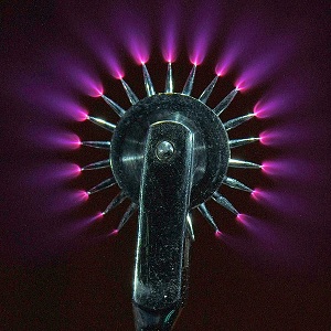
The plasma discharge occurs at the sharp tips of this contraption. To explain this, we consider a configuration of a conductor with a sphere (radius \(R_1\)) connected to another sphere (radius \(R_2>R_1\)) by a wire (length \(\ell\gg R_2\)). Since \(\ell\) is large, we can assume that the potential on the surface of either sphere is independent of the existence of the other sphere. Hence, the potential on the surface of either sphere is given by: \[V_n=\frac{Q_n}{4\pi\varepsilon_0 R_n}\] We have shown earlier that the surface of a conductor must be an equipotential surface, hence we set the potentials on the surfaces of both spheres equal to each other. Cancelling constants yields: \[\frac{Q_1}{R_1}=\frac{Q_2}{R_2}\] Now, when the radius of a sphere is scaled by a factor \(k\), the charge of the sphere is also scaled by \(k\). However, the surface area of the sphere is scaled by a factor \(k^2\). This means that the surface charge density, \(\sigma\), is scaled by a factor of \(\frac{1}{k}\). We consider a Gaussian surface just above an infinitesimally small section of the surface of the conductor, and one just below. Since the conductor is in electrostatic equilibrium, the flux through the surface within the conductor is 0. Hence, by Gauss’ Law: \[E\cdot\textrm{d}A=\frac{\textrm{d}q}{\varepsilon_0}\] Rearranging this gives us an electric field of \(\frac{\sigma}{\varepsilon_0}\). This result was one that I was familiar with and is already on my website.
But the point of this is that the larger sphere has a smaller surface charge density, and since \(\sigma\propto E\), it must have a smaller electric field as well. With a smaller electric field, electrons are less compelled to accelerate to the extent required to ionize atoms in the air causing electrical breakdown and plasma discharge! Hence, smaller spheres with higher curvatures and smaller radii would be needed to produce electric fields strong enough to lead to plasma discharge! This argument extends to all conductors as any conductor’s surface can be represented by an infinite number of osculating circles.
Tough stuff. There’s still lots more to learn. But it’s pretty darn rewarding.